Min Jean Cho

min_jean_cho@brown.edu

Contents

Introduction to Deep Learning Logit and Bayesian Inference Variational Autoencoder (VAE)

Bayesian Inference Bayesian Model Comparison Bayesian Search

Probability and Random Variable Multinomial Distribution and Dirichlet Distribution Linear Probabilistic Model and Linear Regression

Thinking Out Loud

How Artificial Neural Network Mimics Biological Neural Network Towards the Next Generation of Artificial Neural Network EuNet: Artificial Neural Network with Feedback Connections Neural Network for Maximizing Generalization Neural Network for Solving Mathematical Expression

Graph2Seq: Tensor Representation of Directed Acyclic Graph and Its Application to Deep Generative Model for Molecule Generation Task An Analysis of Course Review Data at Brown University Helping VAE by Regularizing Latent Vector

Probability and Random Variable

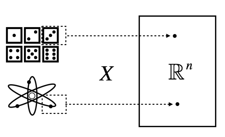
You may have heard of Schrödinger’s cat mentioned in a thought experiment in quantum physics. Briefly, according to the Copenhagen interpretation of quantum mechanics, the cat in a sealed box is simultaneously alive and dead until we open the box and observe the cat. The macrostate of cat (either alive or dead) is determined at the moment we observe the cat. Although not directly applicable, I think the indeterminacy of macrostate in quantum mechanics has some analogy to random variable in probability theory in that the value (\(x\)) of the random (\(X\)) is determined at the moment the random is observed and we say \(x\) is the realization of \(X\).

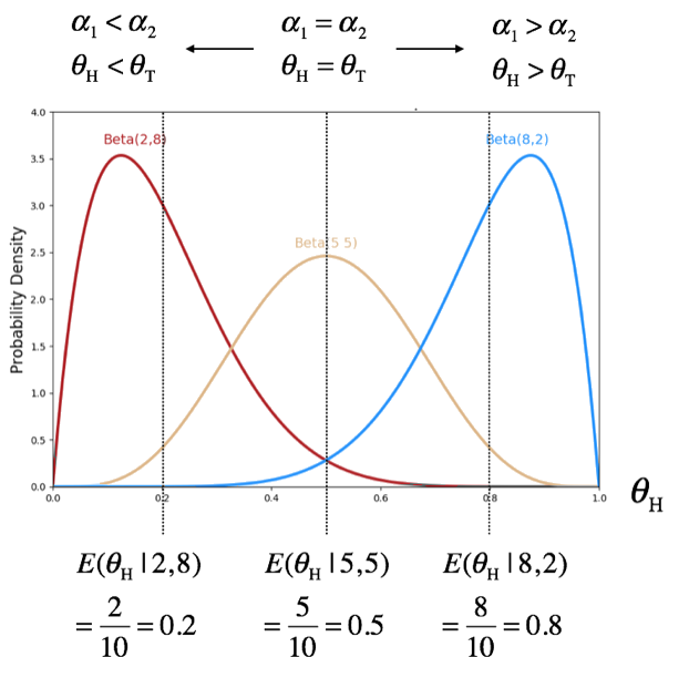
Multinomial Distribution and Dirichlet Distribution

You may remember that Bayesian probability is a belief. We can numerically express our belief using the beta distribution. For example, if we believe a coin is balanced, our belief on this coin’s parameter (\(\theta_T = \theta_H\)) can be expressed using two parameters (\(\alpha_T = \alpha_H\)) of beta distribution such that the expected value of beta RV is \(E(\theta_H|\alpha_1, \alpha_2) = 0.5\).

Bayesian Inference

Considering that Bayesian inference is a process of updating prior (belief), a posterior drawn by observing data becomes the prior for the next time, which is very similar to our brain's learning process. And such update process continues until no more update occurs. Thus, even if we started from a very subjective (or absurd) prior, we will eventually reach an objective posterior. Also, with very big data, both Bayesian approach and frequentist's approach draw the same conclusion, while Bayesian approach is especially useful for small or limited data.

Bayesian Model Comparison

If base compositions of viral sequences and eukaryotic genome sequence is different, the genomic regions that contains viral sequences can be easily detected by using Bayesian model comparison. First, let’s define a DNA sequence \(\mathbf{x}\) with length \(n\) as a string composed of \(n\) independent alphabets \(a \in \mathscr{A} = \{A,T,G,C\}\), that is each sequence position is IID random variables.

Bayesian Search

Bayesian search method has been used for many purposes. A well-known example is the search for a US submarine named USS Scorpion that was lost and found in 1968. Including the lost object search, Bayesian search method can be applied for various areas where pinpointing a target (with trial-and-errors) is required such as optimization of hyperparameters of deep learning models. I will explain the basic algorithm of Bayesian search method using the submarine example.

Linear Probabilistic Model and Linear Regression

The term 'regression' was originally used to describe a biological phenomenon that the heights of descendants of tall ancestors tend to regress down towards a normal average (this phenomenon was called regression toward the mean). Later, the biological regression analysis was developed into a general statistical analysis.

Let’s suppose that we want to fit the simple linear model, \(E(Y) = \beta_0 + \beta_1 x\), to the data set comprised of \(n\) data points (the values of independent variable \(\{x_i \}_{i=1}^n\) as well as the values of dependent variable \(\{y_i \}_{i=1}^n\)). The objective of simple linear regression (SLR) is to estimate \(E(Y)\) using the estimates of parameters.

\[\hat{y} = \widehat{E(Y)} = \hat{\beta_0} + \hat{\beta_1}x\]

Logit and Bayesian Inference

Posterior probability is a sigmoid function of logit \(\psi\). When \(\psi\) is greater than zero, the probability that model is true is greater than 0.5. Considering that the bias term (intercept) \(b=w_0\) is independent from data term \(x_i\), the bias term can be viewed as log prior odds and the weighted sum of \(x_i\), \(\Sigma = \mathbf{w}\mathbf{x}\), can be viewed as log likelihood ratio.

Variational Autoencoder (VAE)

We don’t want \(\mathbf{z}\) to be a point (as in the case of auto encoder) but to be distributed in the latent space such that the distributions of \(\mathbf{z_i}\) from different \(\mathbf{x_i}\) form a continuum.

Thus, what we want to know is the answer to the question "what is the probability distribution of \(\mathbf{z}\), given \(\mathbf{x}\)?" We can answer this question using Bayes’ theorem.

\[P(\mathbf{z}|\mathbf{x}) = \frac{P(\mathbf{x}|\mathbf{z})P(\mathbf{z})}{P(\mathbf{x})} = \frac{P(\mathbf{x}|\mathbf{z})P(\mathbf{z})}{\int P(\mathbf{x}|\mathbf{z})P(\mathbf{z}) d \mathbf{z}}\]

However, the posterior is a very complex function that requires multi-dimensional integration; when the dimensionality is high, analytic solution is virtually impossible

One solution is to use variational inference, where original posterior is replaced with a function (\(Q(\mathbf{z}|\mathbf{x})\)) that is similar to the original posterior but tractable.

\[Q(\mathbf{z}|\mathbf{x}) \approx P(\mathbf{z}|\mathbf{x})\]

How Artificial Neural Network Mimics Biological Neural Network

Dendrites receive signals (in the form of neurotransmitters) from other neurons. When the amount of signals exceeds a threshold, the electrochemical signal is passed to axon terminals. And axon terminals transmit the signals to other neurons through synaptic connection. Brain's learning/memory process involves neurochemical strengthening or weakening synaptic connections between neurons, which is called synaptic plasticity. The synaptic plasticity mainly results from the alteration of the number of neurotransmitter receptors on the dendrite of following neuron; strengthened synaptic connections have more receptors and weakened synaptic connections have less receptors. The weights of 'artificial' neural network mimic the synaptic connections between neurons.

Introduction to Deep Learning

In this article, I explain i) representing neural network with matrices and vectors, ii) learning (optimization of loss function) by gradient descent, and iii) backpropogation. There is also an example at the end to tie all these together.

Towards the Next Generation of Artificial Neural Network

I think that such feedback connections that connects layers to the past will be the next step in deep learning that will make neural networks more like the brain. Now to answer the question asked earlier of why vanishing gradient is a problem in the state-of-the-art deep learning (other than the reason that the derivative becomes zero and the model stops learning), the fundamental reason is that the state-of-the-art neural network is sequentially ordered and gradient needs to backpropogate layer by layer. However, this sequential nature is not at all like the connectivity of neurons in the brain. If there are feedback connections in addition to feedfoward skip connections, is the neural network sequential anymore?

EuNet: Artificial Neural Network with Feedback Connections

Note that the neural network becomes MLP if all gate weights (\(\mathbf{G}_h\)) are zero. And all nodes are inter-connected through \(\mathbf{G}_h \mathbf{x}_{\text{all}}\), although they appeare disconnected at the moment \(i\). Thus, learning the gate weights \(\mathbf{G}_h\) is equivalent to learning the architecture of neural network. I will call the neural network suggested ’EuNet.’ I think that EuNet is a generalization of all possible ANN architectures. For example, convolutional neural network and recurrent neural network can be viewed as a special case of EuNet.

Helping VAE by Regularizing Latent Vector

Such pattern of bubble distribution in a latent space manifests when the complexities of data points to be encoded varies considerably as in the case of ZINC molecules. When the latent space has such pattern, latent space (inter-bubble) interpolation may not be satisfactory due to sudden changes near the center of latent space (dense region). We can observe similar pattern for MNIST digit images. The following figure visualizes the latent space of MNIST digit images after training VAE.

An Analysis of Course Review Data at Brown University

With the Critical Review, course reviews have been a tradition at Brown for many years. We used this data to investigate whether an increase in the number of hours spent on a course resulted in an increase in the expected grade. However, an initial correlation analysis revealed that there was an unintuitive negative correlation between hours spent and grade.

Graph2Seq: Tensor Representation of Directed Acyclic Graph and Its Application to Deep Generative Model for Molecule Generation Task

Generalizable Neural Network for Learning Algebraic Operations Using Quantity Encoding and Abstract Representation of Numbers

Humans have good generalization abilities. For example, children who have learned how to calculate ‘1+2’ and ‘3+5’ can later calculate ‘15 + 23’ and ‘128 × 256.’ They start out understanding the addition with small natural numbers and then later learn a general ‘algorithm’ which is quite explicitly a symbolic computation. Is it possible to develop an artificial intelligence (AI) that can have such generalization ability? If the AI initially trained with limited data for a specific task could easily expand its capability into more general tasks without additional training or modifying its initial architecture, it would be highly beneficial in many fields.

Neural Network for Solving Mathematical Expression

In this article, I propose a neural network (NN) for solving mathematical expression.