An Analysis of Course Review Data at Brown University
With the Critical Review, course reviews have been a tradition at Brown for many years. We used this data to investigate whether an increase in the number of hours spent on a course resulted in an increase in the expected grade. However, an initial correlation analysis revealed that there was an unintuitive negative correlation between hours spent and grade.

I took this photo during the Opening Convocation back in 2016. Time flies when you have fun!
Hypothesis
Minimum study time (X: minhours) is associated with grade received (Y: grade) while controlling the difficulty level (Z: difficult) of course. This hypothesis can be tested using partial correlation coefficient as follows:
\[H_0 : \rho_{XY|Z} = 0\]
\[H_a : \rho_{XY|Z} \ne 0\]
Methods
The course data was scraped from the Critical Review at https://thecriticalreview.org.
View sample data here
Preprocessing the raw dataset (removing class records that do not have the features selected or that contain invalid entries such as "a lot of time, 3-4") resulted in the records of 2774 courses (note that the number of students responses are far greater than 2774 since, in each course, there were mostly far more than 10 students responses).
Features of each course review is shown below:
features = [‘readings','class-materials','difficult','learned', ‘’loved','grading-speed','grading-fairness', ‘effective','efficient','encouraged','passionate', ‘receptive','availableFeedback', ‘Grade’,'minhours','maxhours','class_size']
Course grouping done according to the Critical Review is shown below (e.g., BIOL (biology)):
areas = ["AFRI", "ANTH", "APMA", "ARAB", “ARCH", "BIOL", "CHEM", "CLAS", "CLPS", “COLT", "CSCI", "DEVL", "EAST", "ECON", “EDUC", "EGYT", "ENGL", "ENGN", "ENVS", “ETHN", "FREN", "GEOL", "GNSS", "GRMN", “HIAA", "HIST", "INTL", "ITAL", "JUDS", “KREA", "LITR", "MATH", "MCM", "MDVL", “MES", "MUSC", "NEUR", "PHIL", "PHP", “PHYS", "PLCY", "POBS", "POLS", "RELS", “REMS", "SLAV", "SOC", "SPAN", "TAPS", “URBN", "VISA"]
For each element of feature vector per course, average value of students responses were used. For grade, only "A", "B", and "C" were converted into integers "4", "3", and "2", respectively; "S" and other entries were ignored. *Brown students may take courses for a grade (A,B,C) or satisfactory/no credit (S/NC).
For class_size, the numbers of freshmen, sophomores, juniors, seniors, and graduates were summed.
Since the number of enrolled students (class_size) were different for different courses weighted statistics were used (class_size as weights).
Correlation coefficients were estimated using Pearson sample correlation coefficient (r_xy) calculated from a weighted covariance matrix.
\(H_a\) was tested against \(H_0\) at the significance level of \(\alpha = 0.05\) (two-tailed, t-distribution).
Rationale & Motivation
In the preliminary analysis, correlation coefficients were calculated between all the features and found that minhours and grade showed a weak negative correlation (\(r = -0.16\)), which was unintuitive.
Further inspection of the correlation heat map (Figure 1) revealed that grade showed the highest negative correlation with difficulty (\(r = -0.40\)) and in turn, difficulty showed the highest positive correlation with minhours (\(r = 0.62\)).
Then, it was thought that these three variables (minhours, grade, and difficulty) are inter-related and that difficulty could be a confounding variable that resides between (minhours and grade); the simple correlation coefficient between minhours and grade might not reflect a true relationship between them.
It could be natural to think that study time correlates with grade, but the preliminary analysis showed opposite results. Thus, the partial correlation between minhours and grade while controlling difficulty was focused on.
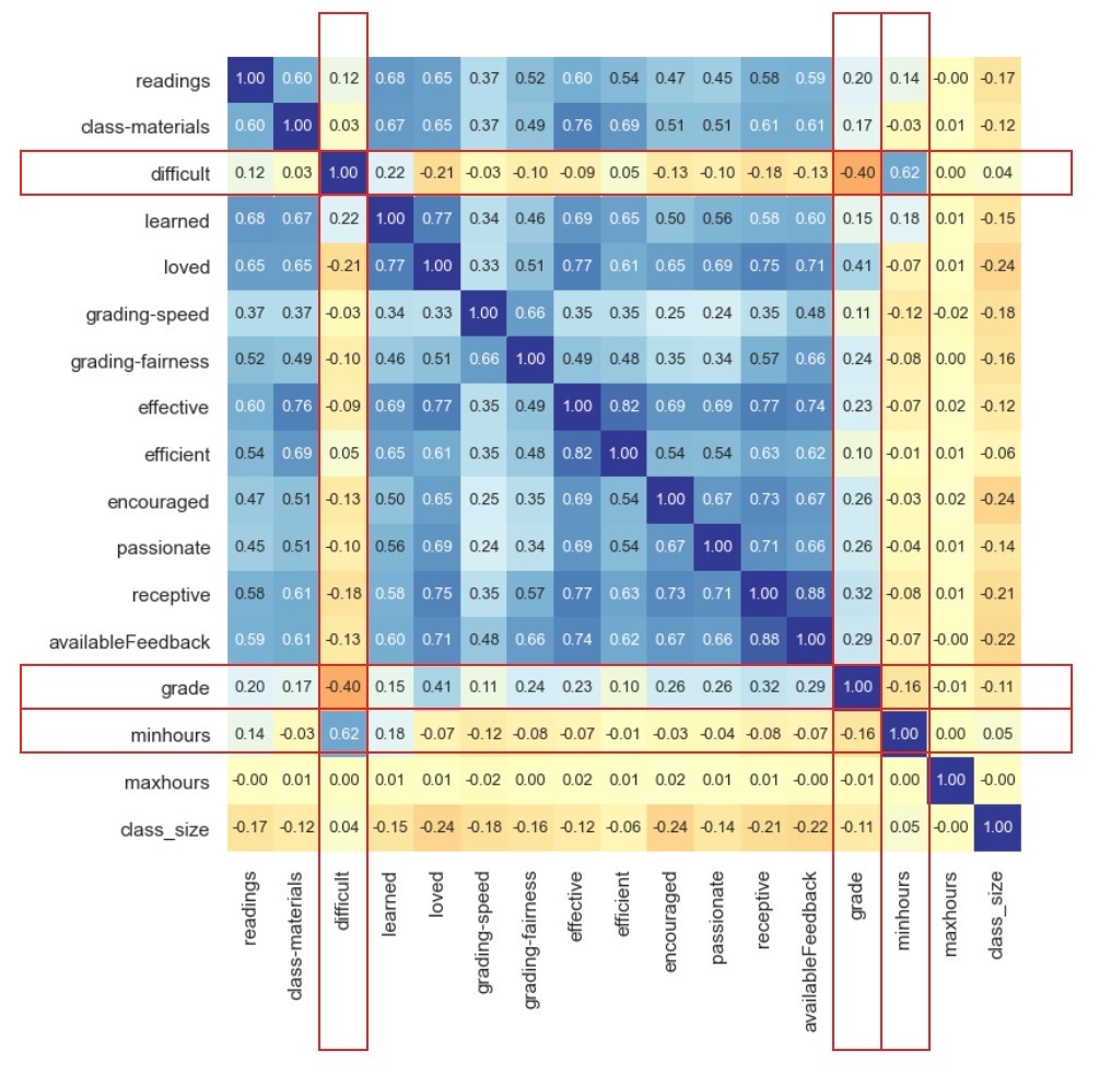
Figure 1. Preliminary correlation analysis (n = 2774). Heat map is based on simple correlation coefficients (Pearson r) calculated from raw data. Blue: positive correlation, red: negative correlation.
Distribution of Data
Since the simple correlation assumes that data points are normally distributed (at least not highly skewed), the distribution of three variables (minhours, grade, and difficult) using weighted histograms (Figure 2) were examined.
Raw dataset showed highly skewed distributions for (minhours and grade).
Outliers were first removed; outliers were defined as those values less than \(Q1 - 1.5 IQR\) or \(Q3 + 1.5 IQR\), where \(Q1\), \(Q3\), and \(IQR\) are first quantile (25 percentile), third quantile (75 percentile), and interquartile range \((Q3 - Q1)\).
After removing the outliers, minhours did not show severe skew but grade still showed skew. In grade variable values, there was a peak at ’4’, which implies that there are some courses in which all students received ’A’ (hereafter referred to as ’all-A courses’). Manual inspection of data showed that the class sizes of most all-A courses are very small.
After applying Box Cox transformation, the skew of grade was in part removed but the peak caused by all-A courses remained.
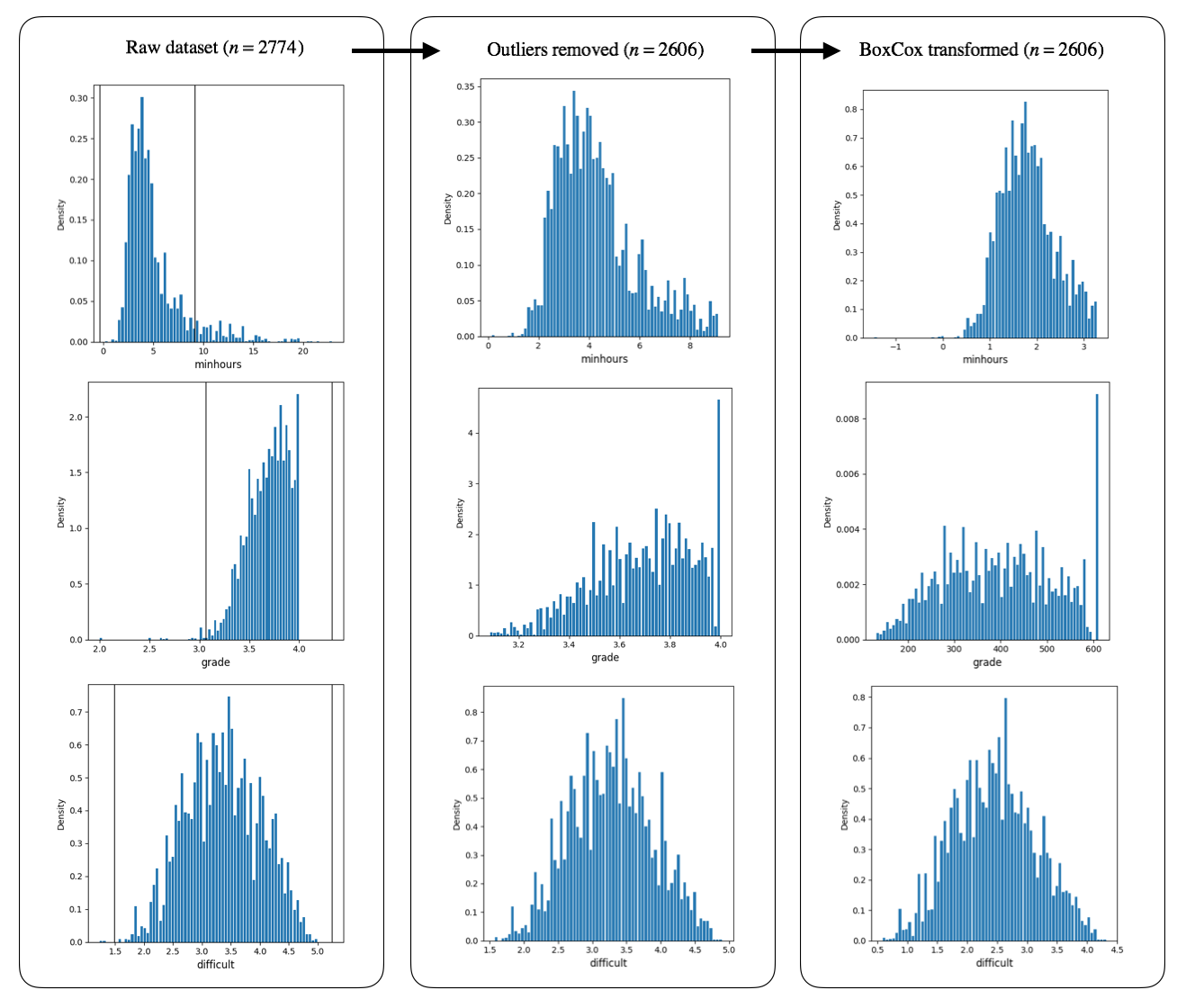
Figure 2. Histogram representation of distributions of raw, outlier-removed, and Box Cox transformed (after outliers removed) datasets. Class sizes were used for weighting the each data point. Vertical lines for raw dataset indicate boundaries for outliers.
Correlation and Partial Correlation
Correlation analysis on outlier-removed dataset was performed (Fig. 3 and 4 and Table 1) and Box Cox transformed dataset (see Fig. 5 and 6 and Table 2) with or without all-A courses. For scatter plots, datasets with all-A courses were used.
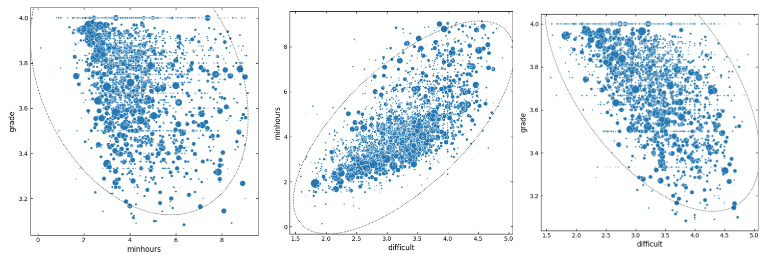
Figure 3. Scatter plot representations of pairwise relationships between minhours, grade, and difficult determined using outlier-removed dataset. All-A courses are included in the dataset. Sizes of markers are scaled relative to the class size. Dotted line indicates confidence ellipse.

Table 1. Correlation analysis using outlier-removed dataset. Correlation coefficients between minhours, grade, and difficult and partial correlation between minhours and grade (while controlling difficult) are shown. p-values are based on t-distributions.
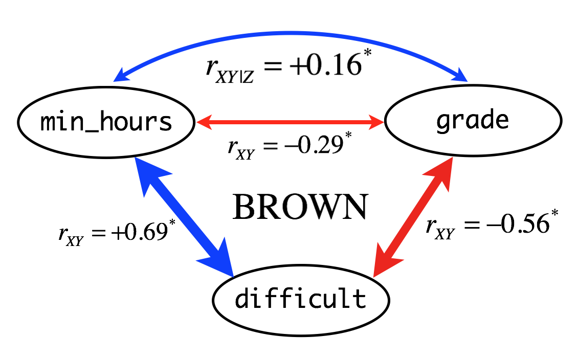
Figure 4. Schematic representation of the relationships between minhours, grade, and difficult. \(r_{XY}\) and \(r_{XY|Z}\) indicate simple correlation (straight line) and partial correlation (curved line) coefficients, respectively. Correlation coefficients are based on outlier-removed dataset with all-A courses. Asterisk indicate significant (p < 0.05) correlation between variables. Widths of arrow lines (positive correlation: blue, negative correlation: red) were scaled approximately relative to correlation coefficients.
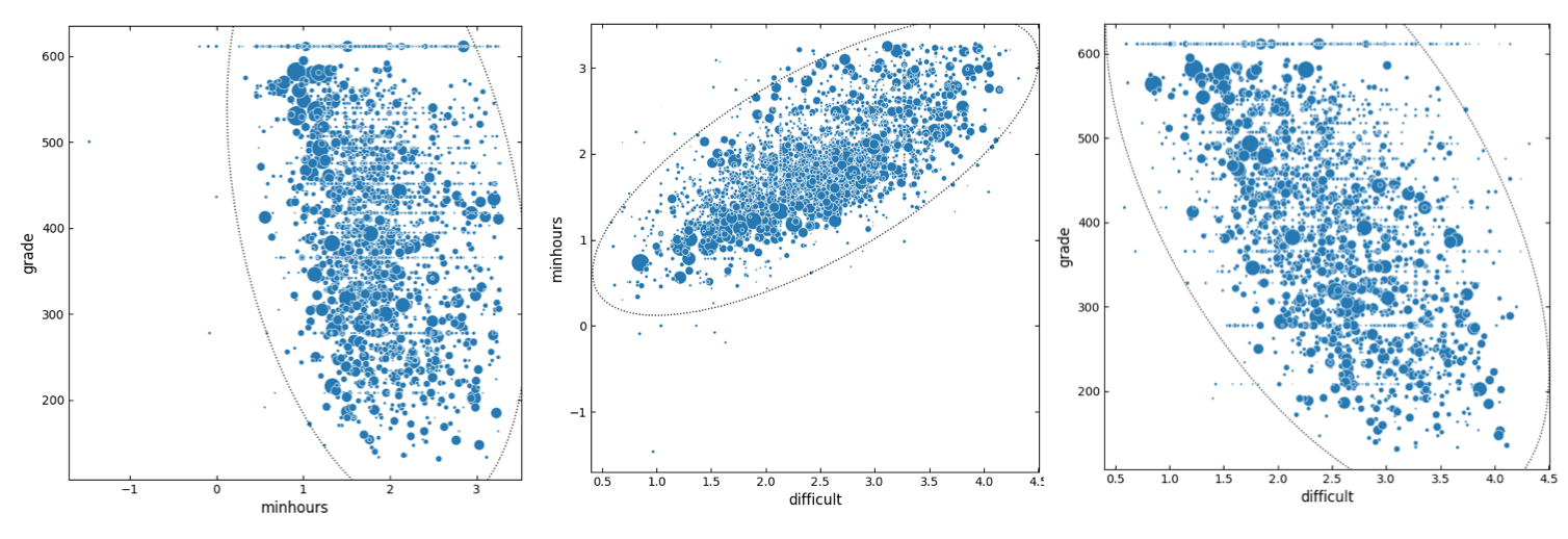
Figure 5. Scatter plot representations of pairwise relationships between minhours, grade, and difficult determined using BoxCox-transformed dataset. All-A courses are included in the dataset. Sizes of markers are scaled relative to the class size. Dotted line indicates confidence ellipse (the radiuses of the ellipse was calculated using 3 X standard deviation, which makes the ellipse enclose ca. 99.7
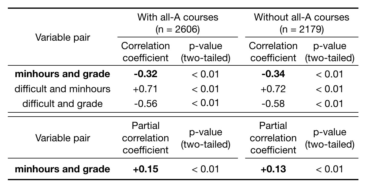
Table 2. Correlation analysis using BoxCox-transformed (after outliers removed) dataset. Correlation coefficients between minhours, grade, and difficult and partial correlation between minhours and grade (while controlling difficult) are shown. p-values are based on t-distributions.
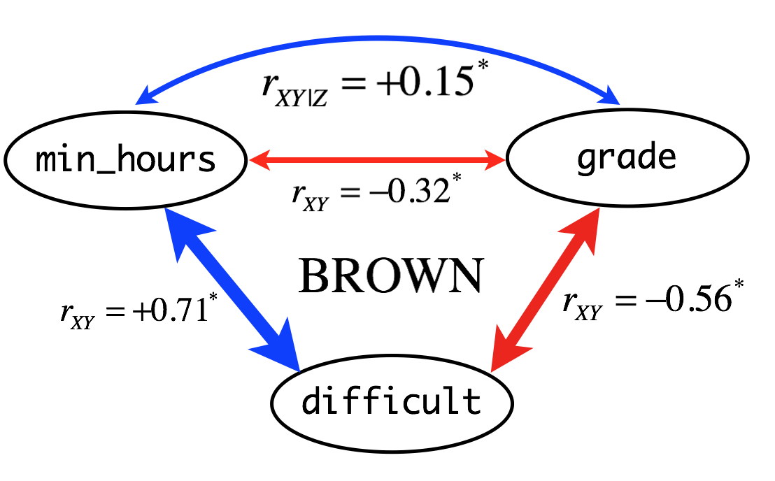
Figure 6. Schematic representation of the relationships between minhours, grade, and difficult. rXY and rXY|Z indicate simple correlation (straight line) and partial correlation (curved line) coefficients, respectively. Correlation coefficients are based on BoxCox-transformed (after outliers removed) dataset with all-A courses. Asterisk indicate significant (p < 0.05) correlation between variables. Widths of arrow lines (positive correlation: blue, negative correlation: red) were scaled approximately relative to correlation coefficients.
Discussion
As shown in Table 1, the correlation analysis results were similar whether including all-A courses or not. This may be due to the use of “weighted" correlation and the class-size being small for the all-A courses (see the size of markers in the top of scatter plots showing grade in Fig 1).
As shown in raw data, correlations between difficult and minhours and between difficult and grade are strong, and negative correlations (\(-0.29\)) between minhours and grade are weak but significant (\(p < 0.05\)).
After controlling difficult, minhours and grade showed positive partial correlation (\(+0.16\)), which is also weak but significant (\(p < 0.05\)).
Thus, H0 was rejected in favor of Ha.
This result implies that the negative correlation between minhours and grade could be due to students spending more time to study difficult courses. The positive partial correlation between minhours and grade suggests that, when the effect of course difficulty is excluded, the more students study the better they can achieve good grades.
Correlation Analysis per course areas
When BoxCox transformation was applied, correlation coefficients are slightly strengthened but overall correlation patterns did not considerably differ from those obtained using outlier-removed datasets. Similarly, exclusion of all-A courses only slightly increased the correlation coefficient. They also did not affect the result of hypothesis test.
Thus, outlier-removed dataset with all-A courses were used for the subsequent analyses. The reason for including all-A courses was that values from these courses are actually not outliers and the effects of these courses could be negligible because the class-size of these courses are very small as shown in scatter plots (Fig. 1) and the use of "weighted" correlations. The reason for not using BoxCox transformation (in spite of that it slightly improves normality of datasets) was due to intention of remaining the scales of the original dataset for the convenience of result interpretations.
Correlation and partial correlation for the groups of courses were investigated to see if overall pattern changes (Simpson’s paradox). For this purpose, outlier-removed dataset with all-A courses were used. The course grouping was done according to Brown’s Critical Review database.
To obtain reliable results, course areas with more than 100 courses were included in this study; they are BIOL (biology), CLPS (Cognitive Linguistic and Psychological Sciences), CSCI (computer science), ECON (economics), ENGN (engineering), HIST (history), MATH (mathematics).
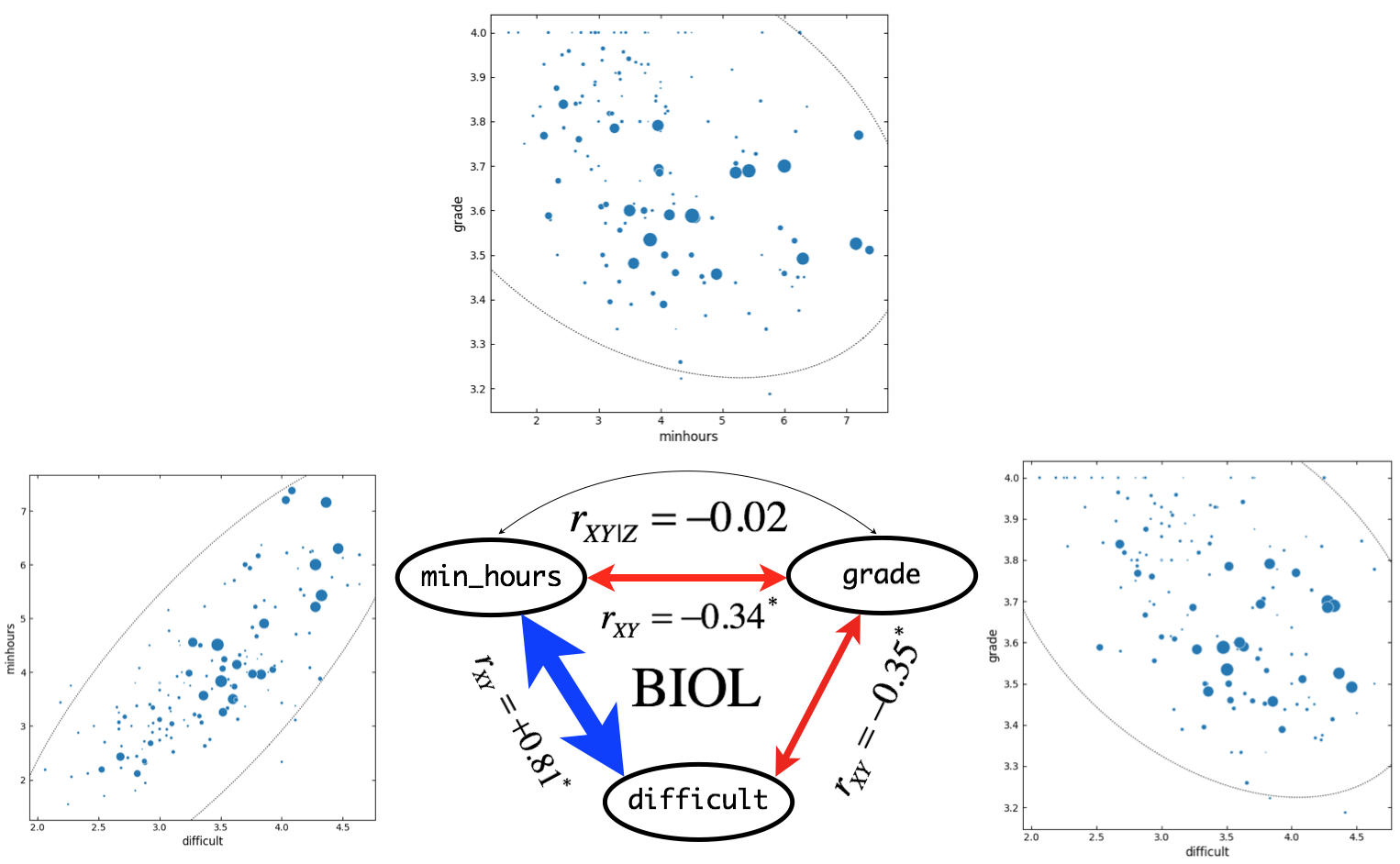
Figure 7. Correlation and partial correlation analyses for BIOL courses (\(n = 147\)). \(r_{XY}\) and \(r_{XY|Z}\) indicate simple correlation (straight line) and partial correlation (curved line) coefficients, respectively. Correlation coefficients are based on outlier-removed dataset with all-A courses. Asterisk indicate significant (\(p < 0.05\)) correlation between variables. Widths of arrow lines (positive correlation: blue, negative correlation: red) were scaled approximately relative to correlation coefficients. In scatter plots, sizes of markers are scaled relative to the class size. Dotted line indicates confidence ellipse.
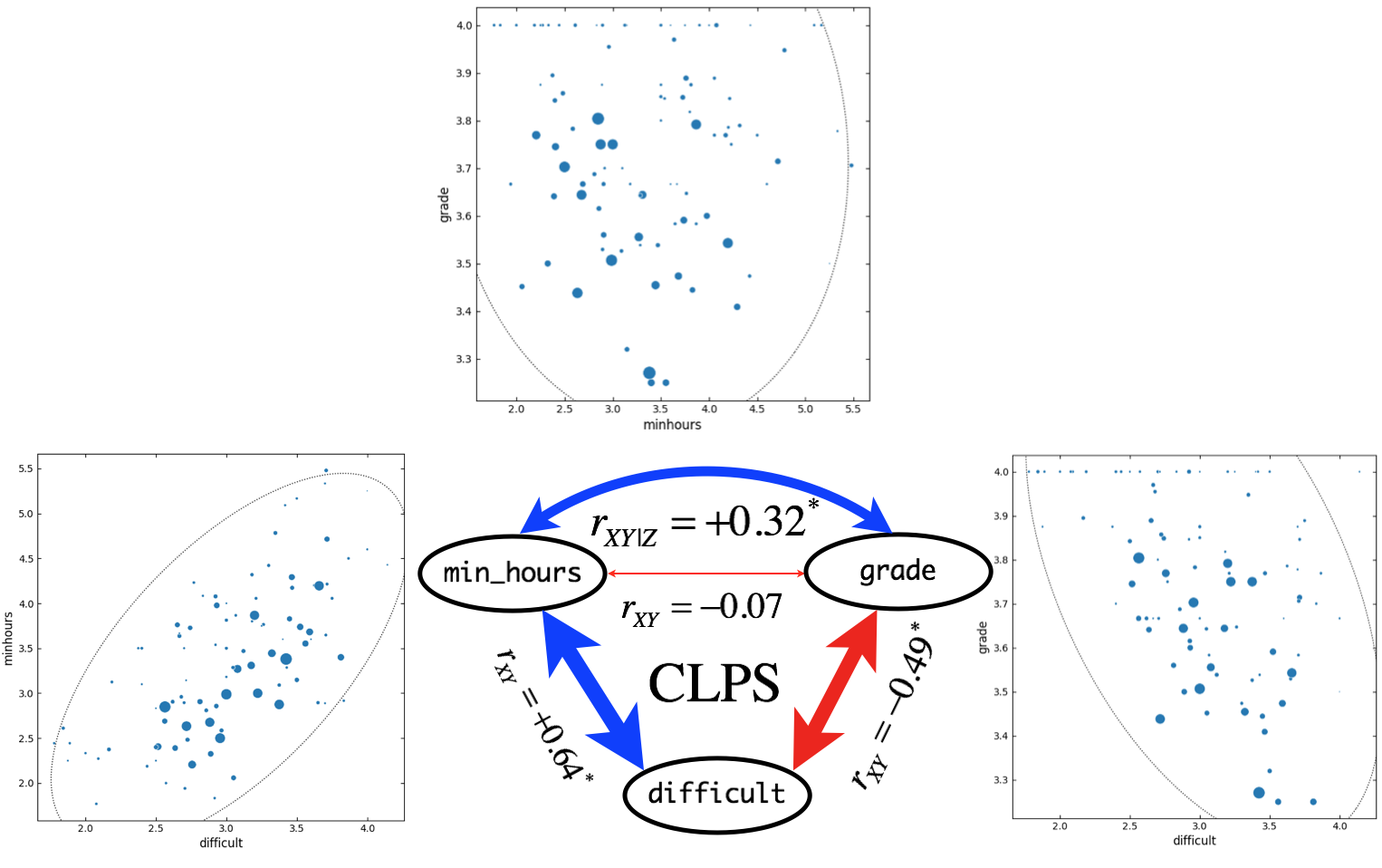
Figure 8. Correlation and partial correlation analyses for CLPS courses (\(n = 100\)). \(r_{XY}\) and \(r_{XY|Z}\) indicate simple correlation (straight line) and partial correlation (curved line) coefficients, respectively. Correlation coefficients are based on outlier-removed dataset with all-A courses. Asterisk indicate significant (\(p < 0.05\)) correlation between variables. Widths of arrow lines (positive correlation: blue, negative correlation: red) were scaled approximately relative to correlation coefficients. In scatter plots, sizes of markers are scaled relative to the class size. Dotted line indicates confidence ellipse.
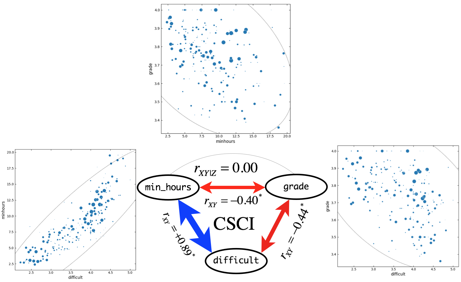
Figure 9. Correlation and partial correlation analyses for CSCI courses (\(n = 202\)). \(r_{XY}\) and \(r_{XY|Z}\) indicate simple correlation (straight line) and partial correlation (curved line) coefficients, respectively. Correlation coefficients are based on outlier-removed dataset with all-A courses. Asterisk indicate significant (\(p < 0.05\)) correlation between variables. Widths of arrow lines (positive correlation: blue, negative correlation: red) were scaled approximately relative to correlation coefficients. In scatter plots, sizes of markers are scaled relative to the class size. Dotted line indicates confidence ellipse.
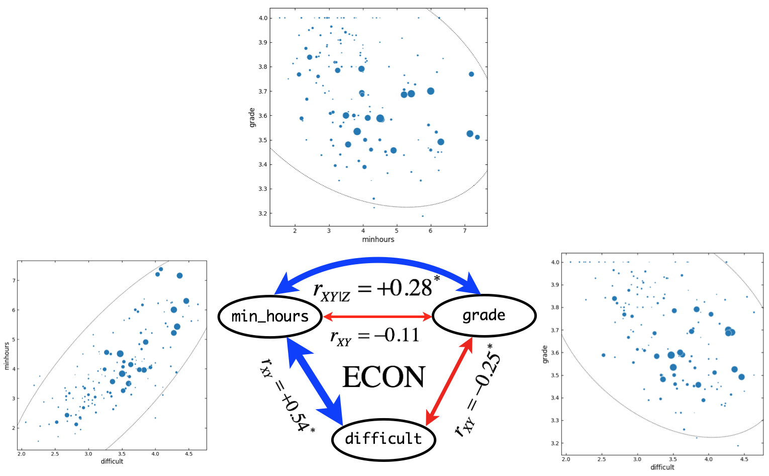
Figure 10. Correlation and partial correlation analyses for ECON courses (\(n = 149\)). \(r_{XY}\) and \(r_{XY|Z}\) indicate simple correlation (straight line) and partial correlation (curved line) coefficients, respectively. Correlation coefficients are based on outlier-removed dataset with all-A courses. Asterisk indicate significant (\(p < 0.05\)) correlation between variables. Widths of arrow lines (positive correlation: blue, negative correlation: red) were scaled approximately relative to correlation coefficients. In scatter plots, sizes of markers are scaled relative to the class size. Dotted line indicates confidence ellipse.
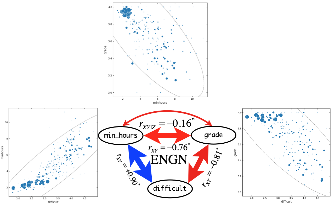
Figure 11. Correlation and partial correlation analyses for ENGN courses (\(n = 216\)). \(r_{XY}\) and \(r_{XY|Z}\) indicate simple correlation (straight line) and partial correlation (curved line) coefficients, respectively. Correlation coefficients are based on outlier-removed dataset with all-A courses. Asterisk indicate significant (\(p < 0.05\)) correlation between variables. Widths of arrow lines (positive correlation: blue, negative correlation: red) were scaled approximately relative to correlation coefficients. In scatter plots, sizes of markers are scaled relative to the class size. Dotted line indicates confidence ellipse.
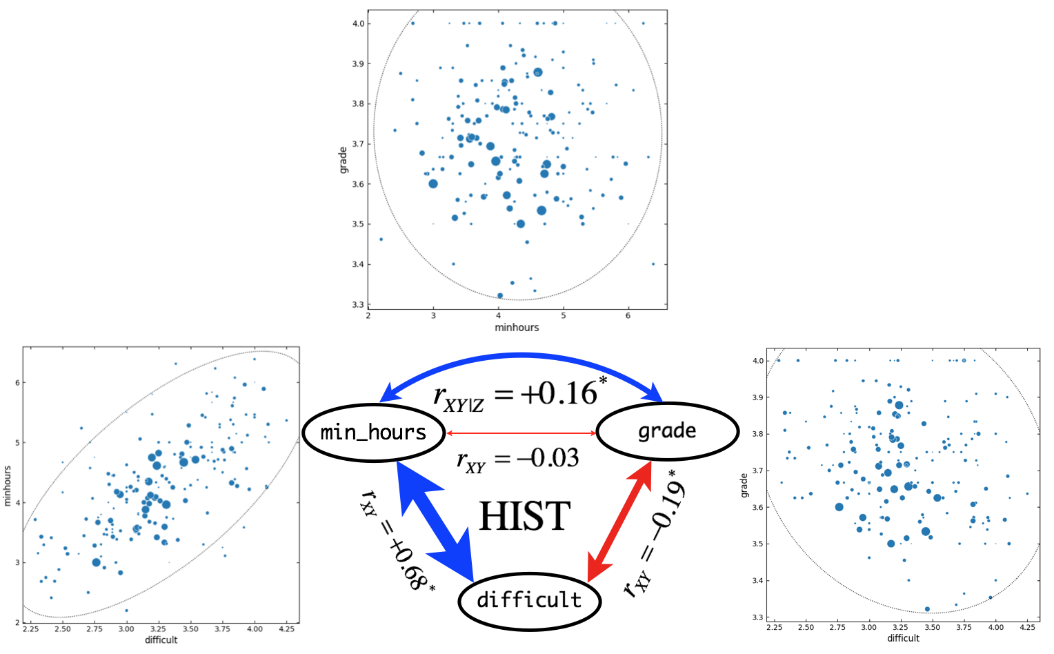
Figure 12. Correlation and partial correlation analyses for HIST courses (\(n = 193\)). \(r_{XY}\) and \(r_{XY|Z}\) indicate simple correlation (straight line) and partial correlation (curved line) coefficients, respectively. Correlation coefficients are based on outlier-removed dataset with all-A courses. Asterisk indicate significant (\(p < 0.05\)) correlation between variables. Widths of arrow lines (positive correlation: blue, negative correlation: red) were scaled approximately relative to correlation coefficients. In scatter plots, sizes of markers are scaled relative to the class size. Dotted line indicates confidence ellipse.

Figure 13. Correlation and partial correlation analyses for MATH courses (\(n = 137\)). \(r_{XY}\) and \(r_{XY|Z}\) indicate simple correlation (straight line) and partial correlation (curved line) coefficients, respectively. Correlation coefficients are based on outlier-removed dataset with all-A courses. Asterisk indicate significant (\(p < 0.05\)) correlation between variables. Widths of arrow lines (positive correlation: blue, negative correlation: red) were scaled approximately relative to correlation coefficients. In scatter plots, sizes of markers are scaled relative to the class size. Dotted line indicates confidence ellipse.
Discussion
For BIOL and CSCI courses, \(H_0\) cannot be rejected. This result implies that in BIOL and CSCI courses, minimum study hours are not associated with grade received. Such results could be due to that BIOL and CSCI courses showed very strong positive correlations (\(r > 0.8\)) between difficult and minhours.
Considering that significant partial correlation can be either positive or negative, it could be better to use one-tailed test. However, in any cases (including all BROWN courses) where \(H_0\) was rejected, \(H_0\) was rejected with big margin. Thus, one-tailed test would not alter the results.
Correlation does not explain causal relationship. However in our case, grade received could be the response/dependent variable and difficult and minhours could be the explaining/independent variable.
Partial correlation coefficient can be calculated while controlling more than two variables. In this study, only one variable (difficult) was controlled. Further studies controlling more variables could provide more comprehensive insight into the relationships between them.
Correlation explains ’linear’ relationships between variables. In this study, by looking at the scatterplots, the variables that showed significant correlation appeared to have linear relationships (Figure 3). However, although not tested thoroughly, it is suspected that the relationship between difficulty and minhours might not be linear but possibly exponential.
Acknowledgement
This was the final project for Brown University CSCI 1951a Data Science during Spring 2020.
Team Members: James Ding, Brendan Le, John Zhou, me
Contribution: John conceived the initial idea of investigating data from the Critical Review. Brendan, John, and James scraped the course data from the Critical Review at https://thecriticalreview.org. I formulated the hypothesis and carried out the experiment and figure presentations. All members discussed the results and made substantial contributions to the project.
Code available at https://github.com/minjeancho/analysis-of-course-review-data-at-brown