Variational Autoencoder (VAE)
Have you ever played a game where there is a deck of cards with random images and one player (player A) randomly picks a card while the other player (player B) cannot see what’s drawn on the card. Player A’s job is to describe the image on the picked card as much as possible to player B. Player B’s job is to re-draw the image as best as possible based on player A’s descriptions.
Autoencoder
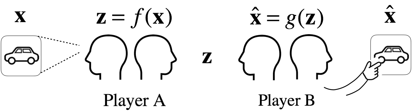
Above diagram shows an autoencoder as a two-player game. Suppose that the car image \(\mathbf{x}\) is composed of \(d\) pixels (\(x\)), i.e., \(d\)-dimensional vector.
\[\mathbf{x} = [x_j]_{j=1}^d \in \mathbb{R}^d\]
After seeing the image \(\mathbf{x}\), player A describes the image using abstract representations of the image (e.g., four doors and four wheels). Let \(p\)-dimensional vector \(\mathbf{z}\) be the abstract descriptions, of which elements (\(z\)) are the abstract features of the image.
Player A is analogous to an encoder, which is a function \(f\) that extracts the abstract features from the image.
\[\mathbf{z} = f(\mathbf{x})\]
Since \(p<<d\), encoder learns the important features of the input image. Player B is analogous to a decoder, which is a function \(g\) that reconstructs the image from \(\mathbf{z}\).
\[\hat{x} = g(\mathbf{z})\]
A referee (analogous to a loss function) can use mean square error (MSE) to score how well player B reconstructed the original image.
\[MSE = \frac{1}{d}\sum_{j=1}^d (x_j- \hat{x_j})^2\]
The goal of player B is to reconstruct the original image, \(\mathbf{x}\), as perfectly as possible, \(\hat{\mathbf{x}}\). But wouldn’t it be interesting as well if player B can also generate similar but different image, \(\tilde{\mathbf{x}}\)? Let’s see the creativity of player B! We talked about images, but how about player B generating new pharmaceuticals based on existing pharmaceuticals (or even new poem!). And here’s where variational autoencoder (VAE) shines.
Variational Autoencoder
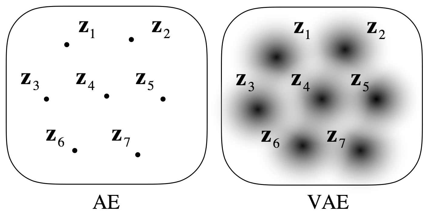
Although there could be parameters (\(\theta\)) involved in the generation of both \(\mathbf{x}\) and \(\mathbf{z}\), suppose we are only interested in \(\mathbf{z}\) that represents \(\mathbf{x}\) in the latent space. Note that we don’t want \(\mathbf{z}\) to be a point (as in the case of auto encoder) but to be distributed in the latent space such that the distributions of \(\mathbf{z_i}\) from different \(\mathbf{x_i}\) form a continuum.
Thus, what we want to know is the answer to the question "what is the probability distribution of \(\mathbf{z}\), given \(\mathbf{x}\)?" We can answer this question using Bayes’ theorem.
\[P(\mathbf{z}|\mathbf{x}) = \frac{P(\mathbf{x}|\mathbf{z})P(\mathbf{z})}{P(\mathbf{x})} = \frac{P(\mathbf{x}|\mathbf{z})P(\mathbf{z})}{\int P(\mathbf{x}|\mathbf{z})P(\mathbf{z}) d \mathbf{z}}\]
The encoder’s job is to return \(\mathbf{z}\) that follows posterior \(P(\mathbf{z}|\mathbf{x})\) from the input \(\mathbf{x}\), that is, the encoder \(f(\mathbf{x})\) samples \(\mathbf{z}\) from \(P(\mathbf{z}|\mathbf{x})\) (actual VAE’s encoder does not sample \(\mathbf{z}\), see reparameterization section).
\[\mathbf{z} = f(\mathbf{x}) \sim P(\mathbf{x}|\mathbf{z})\]
Although the encoder \(f(\mathbf{x})\) does not calculate PMF/PDF of \(P(\mathbf{z}|\mathbf{x})\), the encoder should learn all the parameters (\(\theta\)) required for the Bayesian inference not explicitly shown in the Bayes’ theorem. The decoder’s job is to return (reconstruct) \(\mathbf{x}\), by sampling from likelihood using \(\mathbf{z}\) (actual VAE’s decoder does not sample \(\mathbf{z}\), actual decoder is a deterministic function as explained in the next section).
\[\hat{\mathbf{x}} = g(\mathbf{z}) \sim P(\mathbf{x}|\mathbf{z})\]
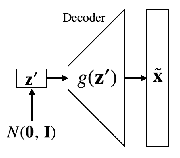
Or we can use \(\mathbf{z}^{'}\) sampled from prior. For the prior distribution, multivariate normal distribution could be a good choice (it is also possible to use other distributions such as multivariate uniform distribution). Using \(\mathbf{z}^{'}\), we can generate \(\tilde{\mathbf{x}}\) that is similar to but different from \(\mathbf{x}\) in training dataset.
\[\tilde{\mathbf{x}} = g(\mathbf{z}^{'}) \sim N(\mathbf{\mu}, \mathbf{\Sigma})\]
Now let’s make neural networks for VAE. Before we begin, we need to note few things. First, transformation \(\mathbf{x} \rightarrow \mathbf{z}\) requires reduction in dimensionality. If the dimensionality of \(\mathbf{z}\) is the same or greater than \(\mathbf{x}\), the encoder can trivially copy \(\mathbf{x}\) to \(\mathbf{z}\). Secondly, decoder should not be a stochastic function but be a deterministic function. In other words, decoder should always reconstruct \(\mathbf{x}\) from \(\mathbf{z}\) only using weights it learned. However, decoder’s outputs can be stochastic if input \(\mathbf{z}\) is sampled from prior (in this case, decoder’s output will be a random variable because input is a random variable even if decoder itself is deterministic). Lastly, posterior is a very complex function that requires multi-dimensional integration; when the dimensionality is high, analytic solution is virtually impossible. One solution is to use MCMC sampling, but if there is a sampling layer, backpropogation cannot be done beyond the sampling layer. Another solution is to use variational inference, where original posterior is replaced with a function (\(Q(\mathbf{z}|\mathbf{x})\)) that is similar to the original posterior but tractable.
\[Q(\mathbf{z}|\mathbf{x}) \approx P(\mathbf{z}|\mathbf{x})\]
The neural network’s objective is to make \(Q(\mathbf{z}|\mathbf{x})\) as much as similar to the original posterior \(P(\mathbf{z}|\mathbf{x})\). At the beginning of training, \(Q(\mathbf{z}|\mathbf{x})\) is not so similar to \(P(\mathbf{z}|\mathbf{x})\). However, as training progresses, \(Q(\mathbf{z}|\mathbf{x})\) becomes similar to \(P(\mathbf{z}|\mathbf{x})\). Therefore, loss function should reflect how much \(Q(\mathbf{z}|\mathbf{x})\) differs from \(P(\mathbf{z}|\mathbf{x})\). And there is a very good metric that can measure the difference between two distributions: relative entropy! The relative entropy is also known as Kullback-Leibler divergence (see appendix for brief introduction of entropy and Kullback-Leibler divergence).
\[D_{KL} = H(Q||P)\]
Nitty-gritty Details of VAE Loss Function
Since KLD \(H(Q||P)\) is an expected value of \(\text{log}(\frac{Q}{P})\) with respect to the distribution \(Q\), our object function, KLD, is as follows:
\[D_{KL}[Q(\mathbf{z}|\mathbf{x})||P(\mathbf{z}|\mathbf{x})] = E_Q \left\{ \text{log} \left[\frac{Q(\mathbf{z}|\mathbf{x})}{P(\mathbf{z}|\mathbf{x})}\right] \right\}\]
Expanding the above equation furthermore,
\[\begin{aligned} D_{KL}[Q(\mathbf{z} | \mathbf{x}) || P(\mathbf{z} | \mathbf{x})] &= E_Q[\text{log} Q(\mathbf{z} | \mathbf{x}) - \text{log} P(\mathbf{z} | \mathbf{x})]\\ &= E_Q[\text{log} Q(\mathbf{z} | \mathbf{x}) - \text{log} P(\mathbf{x} | \mathbf{z}) - \text{log} P(\mathbf{z}) + \text{log} P(\mathbf{x})]\\ &= E_Q[\text{log} Q(\mathbf{z} | \mathbf{x}) - \text{log} P(\mathbf{x} | \mathbf{z}) - \text{log} P(\mathbf{z})] + \text{log} P(\mathbf{x}) \\ &= E_Q[\text{log} Q(\mathbf{z} | \mathbf{x}) - \text{log} P(\mathbf{z})] - E_Q[\text{log} P(\mathbf{x} | \mathbf{z})] + \text{log} P(\mathbf{x})\\ &= D_{KL}[Q(\mathbf{z} | \mathbf{x}) || P(\mathbf{z})] - E_Q[\text{log} P(\mathbf{x} | \mathbf{z})] + \text{log} P(\mathbf{x}) \end{aligned}\]
Note that the marginal likelihood \(P(\mathbf{x}) = \int P(\mathbf{x}|\mathbf{z})P(\mathbf{z})d\mathbf{z}\) is a normalizing constant. Then, we have variational lower bound (VLB) or evidence lower bound (ELBO).
\[\text{ELBO: } \text{log} P(\mathbf{x}) - D_{KL}[Q(\mathbf{z} | \mathbf{x}) || P(\mathbf{z} | \mathbf{x})]\]
\[= -D_{KL}[Q(\mathbf{z} | \mathbf{x}) || P(\mathbf{z})] + E_Q[\text{log} P(\mathbf{x} | \mathbf{z})]\]
Minimizing our original KLD (\(D_{KL}[Q(\mathbf{z}|\mathbf{x})||P(\mathbf{z}|\mathbf{x})]\)) is equivalent to maximizing the ELBO. Then, to maximize ELBO, we need to minimize \(D_{KL}[Q(\mathbf{z}|\mathbf{x})||P(\mathbf{z})]\) and maximize \(E_Q[\text{log}P(\mathbf{x}|\mathbf{z})]\); VAE loss will consist of these two terms.
VAE loss term 1: \(D_{KL}[Q(\mathbf{z}|\mathbf{x})||\text{log}P(\mathbf{z})]\)
Let’s look at in depth the first term we want to minimize. This is the KL divergence our approximation of posterior and the prior. In other words, the neural network needs to approximate posterior as much as similar to the prior. Recall that for the prior we will use is a multivariate normal distribution. Now, let’s make further assumption on the prior that latent dimensions (\(k\) axes) are independent from each other. This assumption is reasonable; the shape of windows (e.g., the first dimension) of car doesn’t need to be dependent on the shape of wheels (e.g., the second dimension). Then the covariance matrix, \(\Sigma\), becomes identity matrix, \(\mathbf{I}\). Additionally, we set \(\mathbf{\mu} = \mathbf{0}\). In other words, each dimension is an independent standard normal (\(\mu_{P,k} =0\) and \(\sigma_{P,k}^2\)). Now, our prior is as follows:
\[P(\mathbf{z})=N(\mathbf{0},\mathbf{I})\]
We will also choose a multivariate normal distribution for \(Q(\mathbf{z}|\mathbf{x})\). Since it is a distribution conditioned on \(\mathbf{x}\), all parameters are functions of \(\mathbf{x}\) : \(\mathbf{\mu}_Q(\mathbf{x})\) and \(\mathbf{\sigma}_Q^2(\mathbf{x})\). But we won’t express \(\mathbf{x}\) for simplicity.
\[Q(\mathbf{z}|\mathbf{x}) = N(\mathbf{\mu_Q}, \text{diag}(\mathbf{\sigma_Q^2}))\]
Now, let’s expand the first term of our VAE loss.
\[\begin{aligned} D_{KL}[Q(\mathbf{z} | \mathbf{x}) || P(\mathbf{z})] &= E_Q\left[\text{log}\frac{N(\mathbf{z}|\mathbf{\mu_Q, \text{diag}(\sigma_Q^2}))}{N(\mathbf{z}|\mathbf{\mu_P, \text{diag}(\sigma_P^2})}\right] \\ &= E_Q\left\{\text{log} \frac{\prod_{k=1}^{p} \frac{1}{\sqrt{2\pi\sigma^2_{Q,k}}}\text{exp}[-\frac{(z_k - \mu_{Q,k})^2}{2\sigma_{Q,k}^2}]}{\prod_{k=1}^{p} \frac{1}{\sqrt{2\pi\sigma^2_{P,k}}}\text{exp}[-\frac{(z_k - \mu_{P,k})^2}{2\sigma_{P,k}^2}]}\right\}\\ &= E_Q\left\{\text{log} \prod_{k=1}^{p} \frac{(\sigma_{Q,k}^2)^{-\frac{1}{2}} \text{exp}[-\frac{(z_k - \mu_{Q,k})^2}{2\sigma_{Q,k}^2}]}{(\sigma_{P,k}^2)^{-\frac{1}{2}} \text{exp}[-\frac{(z_k - \mu_{P,k})^2}{2\sigma_{P,k}^2}]}\right\} \\ &= E_Q\left\{\sum_{k=1}^{p} \text{log} \frac{(\sigma_{Q,k}^2)^{-\frac{1}{2}} \text{exp}[-\frac{(z_k - \mu_{Q,k})^2}{2\sigma_{Q,k}^2}]}{(\sigma_{P,k}^2)^{-\frac{1}{2}} \text{exp}[-\frac{(z_k - \mu_{P,k})^2}{2\sigma_{P,k}^2}]}\right\} \\ &= E_Q\left\{\sum_{k=1}^{p} \left[ -\frac{1}{2}\text{log}\sigma_{Q,k}^2 -\frac{(z_k - \mu_{Q,k})^2}{2\sigma_{Q,k}^2} + \frac{1}{2}\text{log}\sigma_{P,k}^2 + \frac{(z_k - \mu_{P,k})^2}{2\sigma_{P,k}^2} \right] \right\}\\ &= \sum_{k=1}^{p} \left\{ E_Q\left[-\frac{1}{2}\text{log}\sigma_{Q,k}^2 -\frac{(z_k - \mu_{Q,k})^2}{2\sigma_{Q,k}^2} + \frac{1}{2}\text{log}\sigma_{P,k}^2 + \frac{(z_k - \mu_{P,k})^2}{2\sigma_{P,k}^2} \right] \right\}\\ &= \sum_{k=1}^{p}\left\{-\frac{1}{2}\text{log}\sigma_{Q,k}^2 -\frac{E_Q [(z_k - \mu_{Q,k})^2]}{2\sigma_{Q,k}^2} + \frac{1}{2}\text{log}\sigma_{P,k}^2 + \frac{E_Q [(z_k - \mu_{P,k})^2]}{2\sigma_{P,k}^2}\right\}\\ &= \sum_{k=1}^{p}\left\{-\frac{1}{2}\text{log}\sigma_{Q,k}^2 - \frac{\sigma^2_{Q,k}}{2\sigma^2_{Q,k}} + \frac{1}{2}\text{log}\sigma_{P,k}^2 + \frac{E_Q [(z_k - \mu_{P,k})^2]}{2\sigma_{P,k}^2}\right\}\\ &= -\frac{1}{2}\sum_{k=1}^{p}\left\{\text{log}\sigma_{Q,k}^2 + 1 - \text{log}\sigma_{P,k}^2 - \frac{E_Q [(z_k - \mu_{P,k})^2]}{\sigma_{P,k}^2}\right\} \end{aligned}\]
The expectation term in right hand side is
\[\begin{aligned} E_Q [(z_k - \mu_{P,k})^2] &= E_Q\{[(z_k - \mu_{Q,k}) + (\mu_{Q,k} - \mu_{P,k})]\}^2\\ &= E_Q[(z_k - \mu_{Q,k})^2] + 2E_Q[(z_k - \mu_{Q,k})(\mu_{Q,k} - \mu_{P,k})] + E_Q[(\mu_{Q,k} - \mu_{P,k})^2] \\ &= \sigma_{Q,k}^2+ 2(\mu_{Q,k} - \mu_{P,k})[E_Q(z_k) - \mu_{Q,k}] + (\mu_{Q,k} - \mu_{P,k})^2 \\ &= \sigma_{Q,k}^2 + (\mu_{Q,k} - \mu_{P,k})^2 \\ \end{aligned}\]
Recall that \(\mu_{P,k}=0\) and \(\sigma_{P,k}^2=0\) for all \(k\). Putting it together,
\[\begin{aligned} D_{KL}[Q(\vec{z} | \vec{x}) || P(\vec{z})] &= -\frac{1}{2}\sum_{k=1}^{p}\left\{\text{log}\sigma_{Q,k}^2 + 1 - \text{log}\sigma_{P,k}^2 - \frac{\sigma_{Q,k}^2 + (\mu_{Q,k} - \mu_{P,k})^2}{\sigma_{P,k}^2}\right\}\\ &= -\frac{1}{2}\sum_{k=1}^{p}\left\{\text{log}\sigma_{Q,k}^2 +1 - \text{log}1 - \frac{\sigma_{Q,k}^2 + (\mu_{Q,k}-0)^2}{1} \right\} \\ &= -\frac{1}{2}\sum_{k=1}^{p}\left\{\text{log}\sigma_{Q,k}^2 +1 - \sigma_{Q,k}^2 - \mu_{Q,k}^2\right\} \end{aligned}\]
And there we have it, the first term of the VAE loss function.
\[\begin{aligned} L_{KLD} &= D_{KL}[Q(\mathbf{z}|\mathbf{x})||P(\mathbf{z})] \\ &= -\frac{1}{2}\sum_{k=1}^{p}[\text{log}\sigma_{Q,k}^2 +1 - \sigma_{Q,k}^2 - \mu_{Q,k}^2] \end{aligned}\]
VAE loss term 2: \(E_Q[\text{log}P(\mathbf{x}|\mathbf{z})]\)
Let’s now look at in depth the second term we want to maximize. It is the expected value of log likelihood. Considering that likelihood is higher when data represents well what the parameter implies, \(P(\mathbf{x}|\mathbf{z})\) increases when the decoder reconstructs \(\mathbf{x}\) well. Now, what can we use for \(E_Q[\text{log}P(\mathbf{x}|\mathbf{z})]\)? We can use MSE or BCE! (Other loss functions are applicable as well.)
\[L_{Reconstruction} = \frac{1}{d}\sum_{j=1}^d (x_j - \hat{x_j})^2\]
Putting it all together, VAE loss function is as follows:
\[L_{VAE} = L_{KLD} + L_{Reconstruction}\]
The KLD term tries to make latent space (posterior) close to the prior, multivariate normal distribution. But as the latent space is getting very close to multivariate normal, the reconstruction loss term increase, since gathering the regions occupied by different \(\mathbf{z}_i\) at the center of the latent space (near at \(\mathbf{\mu}_Q = \mathbf{0}\)) could hinder the reconstruction (although it may improve interpolation). And reconstruction loss term prevents such result in dense overlapping. Thus, the two terms balance each other.
Reparameterization Trick
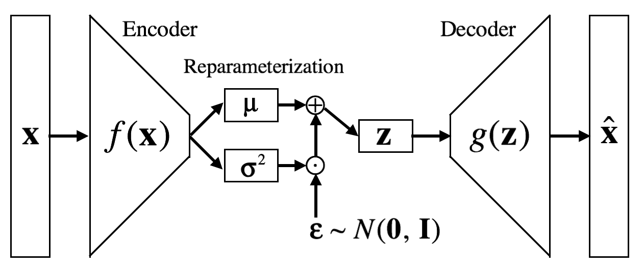
I said earlier that error backpropogation cannot go beyond sampling layer. But we want to sample \(\mathbf{z}\) from \(Q(\mathbf{z}|\mathbf{x})\). Then how do we backpropogate? There is a trick. We’ll let the encoder output the mean and variance of each \(\mathbf{z}\), which indicates the location and range of a region occupied by \(\mathbf{z}\) in the latent space.
\[[\mathbf{\mu}_{\mathbf{z}\sim Q}, \text{log}\mathbf{\sigma}_{\mathbf{z} \sim Q}^2] = f(\mathbf{x})\]
Then random noises sampled from normal distribution are added as follows:
\[\mathbf{z} = \mathbf{\mu}_{\mathbf{z}\sim Q} + \mathbf{\sigma}_{\mathbf{z}\sim Q}^2 \mathbf{\epsilon}, \epsilon \sim N(\mathbf{0}, \mathbf{I})\]
This technique is called reparameterization trick. It makes as if \(\mathbf{z}\) is sampled from posterior.
Summary
VAE architecture is summarized in following diagram.
After training encoder and decoder, \(\mathbf{z}^{'}\) can be sampled from the prior to generate novel output \(\tilde{\mathbf{x}}\).