Introduction to Deep Learning
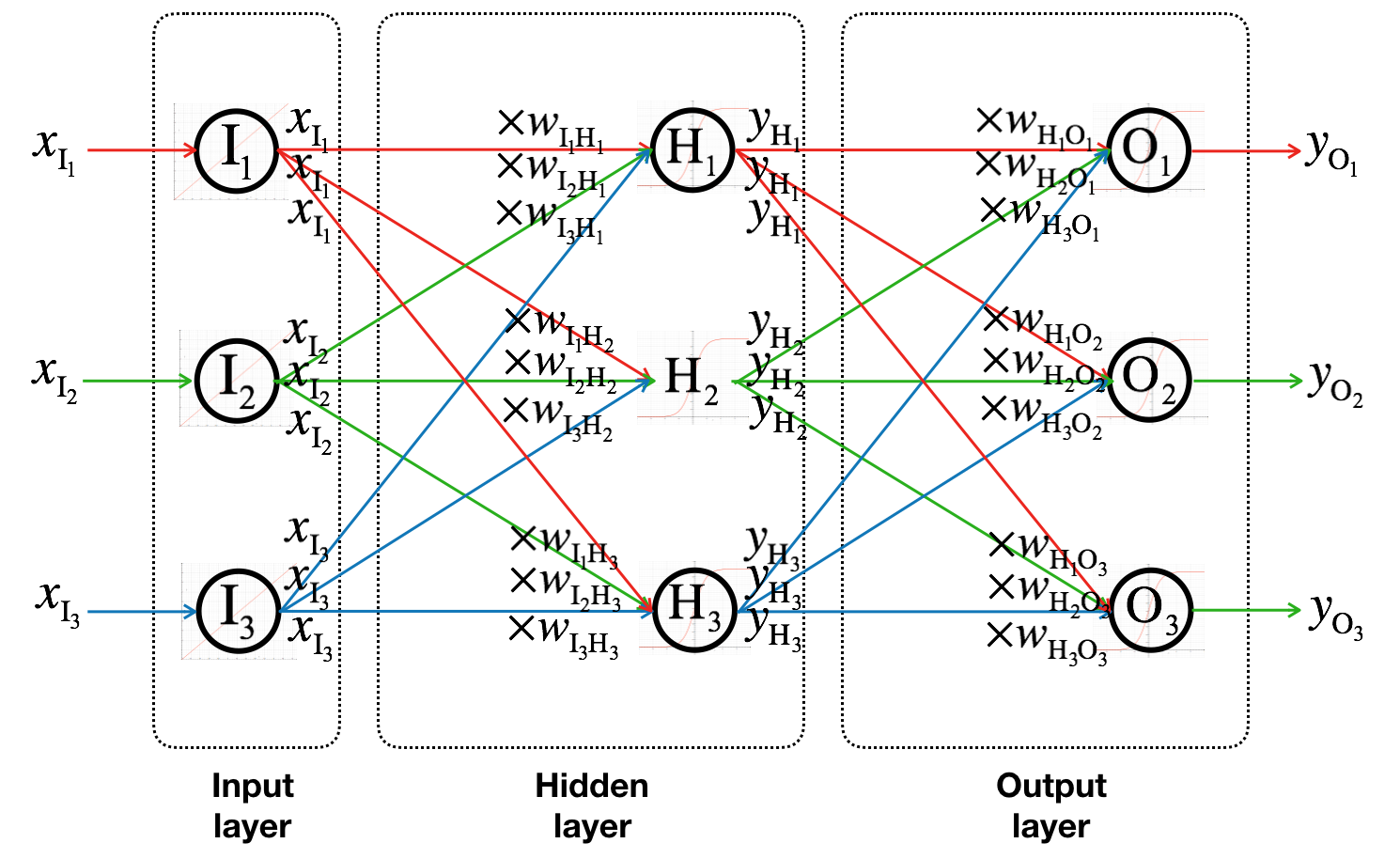
In the previous article, we have made a simple three-layer artificial neural network. The first layer is input layer composed of sensory neurons, each of which has linear activation function: \(y_I = x_I\). And the second (hidden) and the third (output) layers are composed of perceptive neurons, each of which has sigmoid activation function: \(y_H = \sigma(x_H)\) and \(y_O = \sigma(x_O)\).
In this article, I explain i) representing neural network with matrices and vectors, ii) learning (optimization of loss function) by gradient descent, and iii) backpropogation. There is also an example at the end to tie all these together.
Neural Network as Matrices and Vectors
Let’s see how the input signals (\(x_{I_1}\), \(x_{I_2}\), and \(x_{I_3}\)) are transformed to outputs (\(y_{H_1}\), \(y_{H_2}\), and \(y_{H_3}\)) of hidden layer.
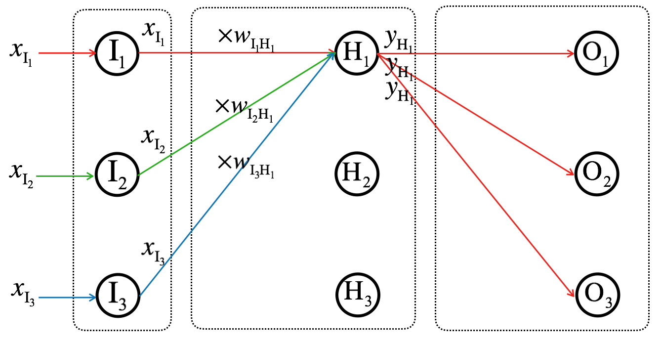
\[\Sigma_{H_1} = x_{I_1}w_{I_1,H_1} + x_{I_2}w_{I_2,H_1} + x_{I_3}w_{I_3,H_1} = \sum_{k=1}^{3} x_{I_k}w_{I_k,H_1}\]
We can represent \(\Sigma_{H_1}\), \(\Sigma_{H_2}\), and \(\Sigma_{H_3}\) using vector multiplications (dot product):
\[\Sigma_{H_1} = % \begin{bmatrix} w_{I_1,H_1} & w_{I_2,H_1} & w_{I_3,H_1} \end{bmatrix} % \begin{bmatrix} x_{I_1} \\ x_{I_2} \\ x_{I_3} \\ \end{bmatrix}\]
\[\Sigma_{H_2} = % \begin{bmatrix} w_{I_1,H_2} & w_{I_2,H_2} & w_{I_3,H_2} \end{bmatrix} % \begin{bmatrix} x_{I_1} \\ x_{I_2} \\ x_{I_3} \\ \end{bmatrix}\]
\[\Sigma_{H_3} = % \begin{bmatrix} w_{I_1,H_3} & w_{I_2,H_3} & w_{I_3,H_3} \end{bmatrix} % \begin{bmatrix} x_{I_1} \\ x_{I_2} \\ x_{I_3} \\ \end{bmatrix}\]
Putting it all together with the bias term,
\[\begin{bmatrix} \Sigma_{H_1} \\ \Sigma_{H_2} \\ \Sigma_{H_3} \\ \end{bmatrix} = % \begin{bmatrix} w_{I_1,H_1} & w_{I_2,H_1} & w_{I_3,H_1} \\ w_{I_1,H_2} & w_{I_2,H_2} & w_{I_3,H_2} \\ w_{I_1,H_3} & w_{I_2,H_3} & w_{I_3,H_3} \end{bmatrix} % \begin{bmatrix} x_{I_1} \\ x_{I_2} \\ x_{I_3} \\ \end{bmatrix} + % \begin{bmatrix} b_{H_1} \\ b_{H_2} \\ b_{H_3} \\ \end{bmatrix}\]
Then using matrix notation,
\[\mathbf{\Sigma_{H}} = \mathbf{W_{IH}}\mathbf{x_I} + \mathbf{b_H}\]
The bias terms can be incorporated into to the weight matrix \(\mathbf{W}\) by letting \(w_{I_0H_k} = b_{H_k}\) and \(x_{I_0}=1\) as follows:
\[\begin{bmatrix} \Sigma_{H_1} \\ \Sigma_{H_2} \\ \Sigma_{H_3} \end{bmatrix} % = \begin{bmatrix} b_{H_1} & w_{I_1H_1} & w_{I_2H_1} & w_{I_3H_1} \\ b_{H_2} & w_{I_1H_2} & w_{I_2H_2} & w_{I_3H_2} \\ b_{H_3} & w_{I_1H_3} & w_{I_2H_3} & w_{I_3H_3} \end{bmatrix} % \begin{bmatrix} 1 \\ x_{I_1} \\ x_{I_2} \\ x_{I_3} \end{bmatrix}\]
From now on, I will not show the bias terms explicitly.
\[\mathbf{\Sigma_H} = \mathbf{W_{IH}}\mathbf{x_I}\]
Then, the outputs of the hidden layers are as follows:
\[\mathbf{y_H} % = \begin{bmatrix} y_{H_1} \\ y_{H_2} \\ y_{H_3} \end{bmatrix} % = \sigma \left( \begin{bmatrix} \Sigma_{H_1} \\ \Sigma_{H_2} \\ \Sigma_{H_3} \end{bmatrix} \right)\]
With matrix notation,
\[\mathbf{y_H} = \sigma(\mathbf{\Sigma_H})\]
If we want to reduce the dimensionality of the output, we use the weight matrix with the reduced number of rows (intended dimensionality) as follows.
\[\begin{bmatrix} \Sigma_{H_1} \\ \Sigma_{H_2} \end{bmatrix} % = \begin{bmatrix} b_{H_1} & w_{I_1H_1} & w_{I_2H_1} & w_{I_3H_1} \\ b_{H_2} & w_{I_1H_2} & w_{I_2H_2} & w_{I_3H_2} \end{bmatrix} % \begin{bmatrix} 1 \\ x_{I_1} \\ x_{I_2} \\ x_{I_3} \end{bmatrix}\]
Let’s now see how the outputs of hidden layer (\(y_{H_1}\), \(y_{H_2}\), and \(y_{H_3}\)) are transformed to outputs of final/output layer (\(y_{O_1}\), \(y_{O_2}\), and \(y_{O_3}\)).
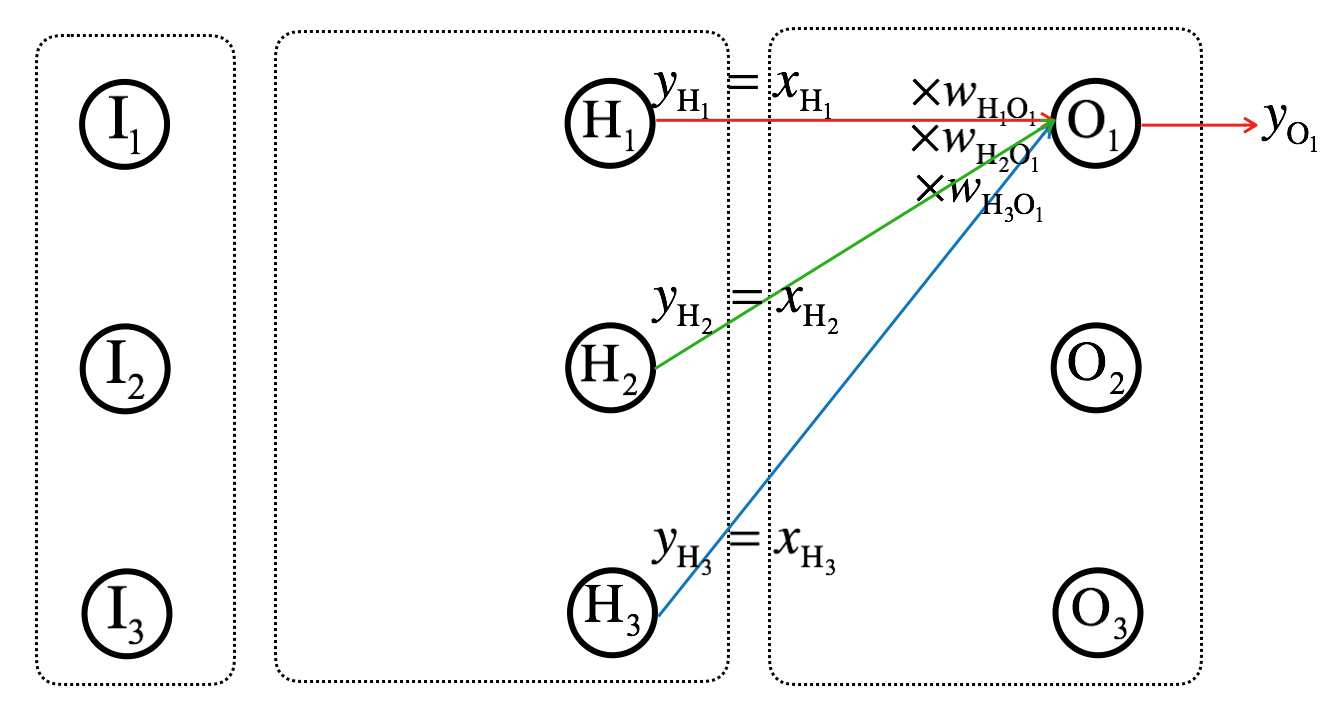
Because the outputs of hidden layer will be the input of output layer, I will let
\[\mathbf{x_H} = \mathbf{y_H}\]
Then, similarly as before,
\[\mathbf{\Sigma_{O}} = \mathbf{W_{HO}} \mathbf{x_H}\]
\[\mathbf{y_O} = \sigma(\mathbf{\Sigma_O})\]
Finally putting it all together from the neural network inputs to outputs,
\[\mathbf{y_O} = \sigma(\mathbf{W_{HO}}\sigma(\mathbf{W_{IH} x_{I}}))\]
As a reminder, \(\mathbf{x_I}\) is the input vector, \(\mathbf{y_O}\) is the output vector, and \(\mathbf{W}\) is the weight matrix. \(\mathbf{W}\) is the parameter of the neural network, and the elements of \(\mathbf{W}\) (arbitrary values at the beginning) is updated during training.
In this example, we had a simple, three-layer neural network. But we can have much deeper neural network as well:
\[\mathbf{y_O} = \sigma(\mathbf{W_{H_NO}} ... \sigma(\mathbf{W_{H_2H3}} \sigma(\mathbf{W_{H_1H2}} \sigma(\mathbf{W_{IH_1}x_I}))))))\]
Loss and optimization
\(\mathbf{y_o}\) is also called neural network’s prediction of ground truth values. In case of supervised learning, to make the neural network learn its weights, we need to teach the neural network using training dataset (inputs, \(\mathbf{x_I}\)) and true values of outputs (ground truth, \(\mathbf{y_T}\)). And ’loss (error)’ is a metric that measures how bad the neural network predictions are. Thus, learning requires minimizing the loss.
I will briefly explain a gradient descent method for optimizing (finding minimum or maximum of a function) loss function. Let, \(e\) be the error (loss) and let \(w\) be the parameter of which we want to find its value (\(w^{*}\)) that would result in the lowest \(e\). Then, we can write our loss function as follows:
\[e=f(w)\]
Starting from an arbitrary initial value, \(w^{(0)}\), we will find \(w^{*}\) by adding some small values to \(w^{(i)}\) through iterations as follows:
\[w^{(i+1)} = w^{(i)} + \Delta w^{(i)}, i=0,1,2,...\]
Let’s first think of the sign of \(\Delta w^{(i)}\). If \(w^{(i)}\) is lower than \(w^{*}\), the sign of \(\Delta w^{(i)}\) should be positive, otherwise it should be negative. Thus, the sign of \(\Delta w^{(i)}\) is opposite of the sign of the derivative of the loss function.
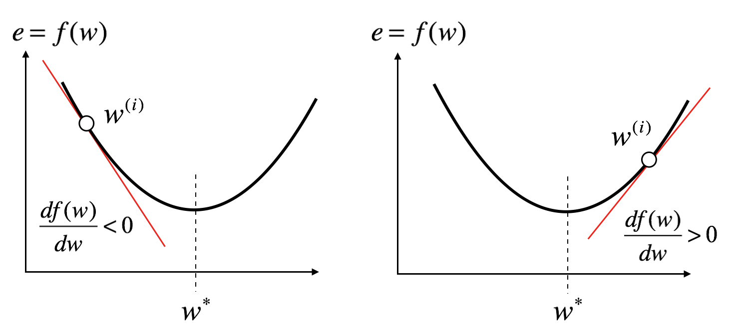
Also the magnitude of \(\Delta w^{(i)}\) is proportional to the derivative. Then, we can write the parameter update equation as follows:
\[w^{(i+1)} = w^{(i)} - \alpha \frac{df(w^{(i)})}{dw^{(i)}}\]
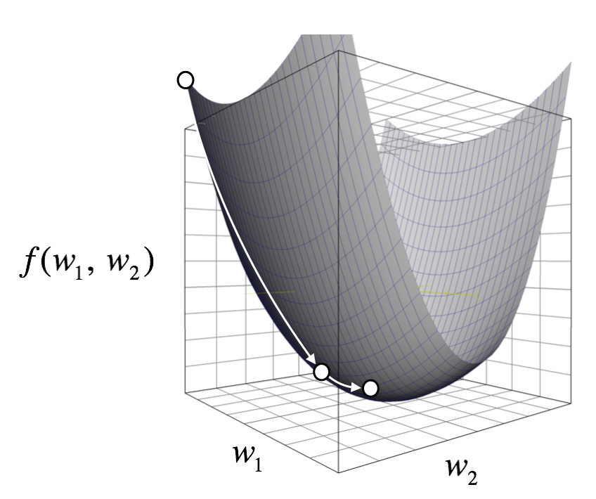
\(\alpha\) is called the learning rate, which determines the amount of value to be updated per iteration. If \(\alpha\) is too large, we may not find the minimum because \(w^{(i+1)}\) could leap over the minimum and swing near the minimum. If \(\alpha\) is too small, the learning will be very slow. The following diagram shows multivariate version of the gradient descent method.
What should the loss function be? There’s a lot of different loss functions one could use. Some of the well-known loss functions are mean squared error (MSE) loss, cross entropy (CE) loss, and binary cross entropy (BCE) loss. Or one could come up with their own loss function as long as it’s differentiable (why? see below). In this article, we’ll use the sum of squared error (SSE) loss.
\[e_k = y_{T_k} - y_{O_k}\]
\[SSE = \sum_{k=1}^{K}e_{k}^{2} = \sum_{k=1}^{K} (y_{T_k} - y_{O_k})^2\]
Now we have our loss function defined. Let’s see how the weights are learned/updated.
Backpropagation
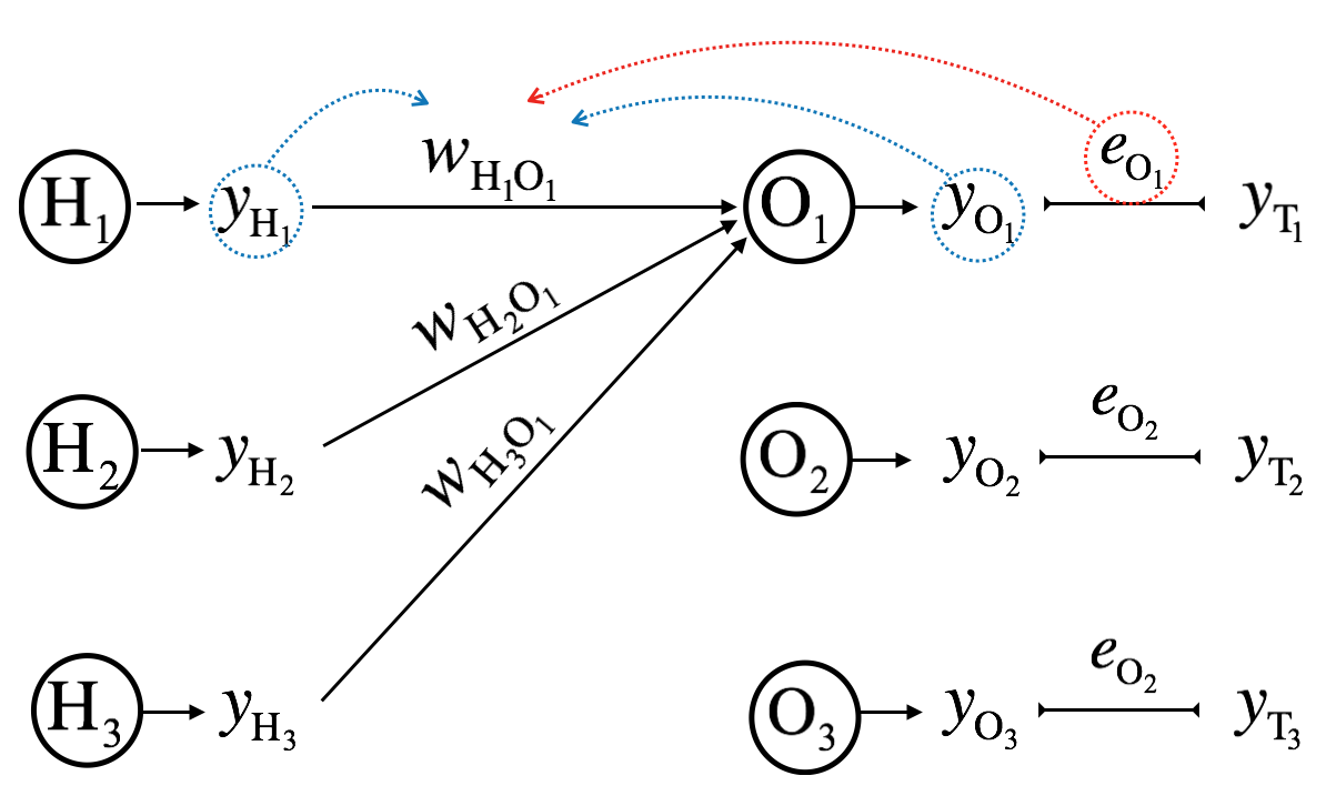
Let’s first see how we update a single weight term of output layer, \(w_{H_jO_k}^{(i+1)}\), at the \(i^{th}\) iteration.
\[\mathbf{W_{HO}^{(i)}} = \begin{bmatrix} w_{H_1O_1}^{(i)} & w_{H_2O_1}^{(i)} & w_{H_3O_1}^{(i)} \\ w_{H_1O_2}^{(i)} & w_{H_2O_2}^{(i)} & w_{H_3O_2}^{(i)} \\ w_{H_1O_3}^{(i)} & w_{H_2O_3}^{(i)} & w_{H_3O_3}^{(i)} \end{bmatrix}\]
\[\mathbf{e_O^{(i)}} = \mathbf{y_T} - \mathbf{y_O^{(i)}} = \begin{bmatrix} y_{T_1} - y_{O_1}^{(i)} \\ y_{T_2} - y_{O_2}^{(i)} \\ y_{T_3} - y_{O_3}^{(i)} \end{bmatrix}\]
\[w_{H_jO_k}^{(i+1)} = w_{H_jO_k}^{(i)} - \alpha \frac{\partial SSE^{(i)}}{\partial w_{H_jO_k}^{(i)}}\]
Here, we will define the error as \(e_{O_k} = y_{T_k} - y_{O_k}\) in order to explicitly represent that it is the error of the output layer. SSE is a function of weights, and we need to calculate partial derivative of it.
\[\begin{aligned} \frac{\partial SSE^{(i)}}{\partial w_{H_jO_k}^{(i)}} &= \frac{\partial}{\partial w_{H_jO_k}^{(i)}}\sum_{z=1}^{K} (y_{T_z} - y_{O_z}^{(i)})^2 \\ &= \frac{\partial y_{O_k}^{(i)}}{\partial w_{H_jO_k}^{(i)}} \frac{\partial}{\partial y_{O_k}^{(i)}}\sum_{z=1}^{K} (y_{T_z} - y_{O_z}^{(i)})^2\\ &= \frac{\partial y_{O_k}^{(i)}}{\partial w_{H_jO_k}^{(i)}} \frac{\partial}{\partial y_{O_k}^{(i)}}[(y_{T_k} - y_{O_k}^{(i)})^2 + \sum_{z \neq k}^{K} (y_{T_z} - y_{O_z}^{(i)})^2]\\ &= \frac{\partial y_{O_k}^{(i)}}{\partial w_{H_jO_k}^{(i)}} \frac{\partial}{\partial y_{O_k}^{(i)}}[(y_{T_k} - y_{O_k}^{(i)})^2]\\ &= \frac{\partial y_{O_k}^{(i)}}{\partial w_{H_jO_k}^{(i)}} 2(y_{T_k} - y_{O_k}^{(i)})(-1)\\ &= -2e_{O_k}^{(i)} \frac{\partial y_{O_k}^{(i)}}{\partial w_{H_jO_k}^{(i)}}\\ &= -2e_{O_k}^{(i)} \frac{\partial \sigma(\Sigma_{O_k}^{(i)})}{\partial w_{H_jO_k}^{(i)}}\\ &= -2e_{O_k}^{(i)}\sigma(\Sigma_{O_k}^{(i)})[(1-\sigma(\Sigma_{O_k}^{(i)})]\frac{\partial \Sigma_{O_k}^{(i)}}{\partial w_{H_jO_k}^{(i)}} \hspace{80pt} \frac{\partial \sigma(f(x))}{\partial x} = \sigma(f(x))[1-\sigma(f(x))]\frac{\partial f(x)}{\partial x} \text{ by chain rule}\\ &= -2e_{O_k}^{(i)}\sigma(\Sigma_{O_k}^{(i)})[(1-\sigma(\Sigma_{O_k}^{(i)})]\frac{\partial}{\partial w_{H_jO_k}^{(i)}}\sum_{z=1}^{M}w_{H_zO_k}^{(i)}y_{H_z}^{(i)}\\ &= -2e_{O_k}^{(i)}\sigma(\Sigma_{O_k}^{(i)})[(1-\sigma(\Sigma_{O_k}^{(i)})]\frac{\partial}{\partial w_{H_jO_k}^{(i)}} [w_{H_jO_k}^{(i)}y_{H_j}^{(i)} + \sum_{z \ne j}^{M}w_{H_zO_k}^{(i)}y_{H_z}^{(i)}]\\ &= -2e_{O_k}^{(i)}\sigma(\Sigma_{O_k}^{(i)})[(1-\sigma(\Sigma_{O_k}^{(i)})]y_{H_j}^{(i)}\\ &= -2e_{O_k}^{(i)}y_{O_k}^{(i)}[(1-y_{O_k}^{(i)})]y_{H_j}^{(i)} \end{aligned}\]
Putting it together,
\[w_{H_jO_k}^{(i+1)} = w_{H_jO_k}^{(i)} + \alpha[2e_{O_k}^{(i)}y_{O_k}^{(i)}[(1-y_{O_k}^{(i)})]y_{H_j}^{(i)}]\]
For simplicity, the constant ’2’ can be incorporated into \(\alpha\). Thus,
\[\Delta \mathbf{W_{HO}^{(i)}}= \alpha \begin{bmatrix} e_{O_1}^{(i)} \\ e_{O_2}^{(i)} \\ e_{O_3}^{(i)} \end{bmatrix} \begin{bmatrix} y_{O_1}^{(i)} \\ y_{O_2}^{(i)} \\ y_{O_3}^{(i)} \end{bmatrix} \begin{bmatrix} 1-y_{O_1}^{(i)} \\ 1-y_{O_2}^{(i)} \\ 1-y_{O_3}^{(i)} \end{bmatrix} \begin{bmatrix} y_{H_1}^{(i)} && y_{H_2}^{(i)} && y_{H_3}^{(i)} \end{bmatrix}\]
We’ve so far updated the weights of the output layer. How do we update the weights of the hidden layer? It is quiet similar:
\[\mathbf{W_{IH}^{(i+1)}} = \mathbf{W_{IH}^{(i)}} + \Delta \mathbf{W_{IH}^{(i)}}\]
\[\begin{equation} \begin{aligned} \Delta \mathbf{W_{IH}^{(i)}} &= \alpha \mathbf{e_{H}^{(i)}} \mathbf{y_{H}^{(i)}} \mathbf{(1- y_{H}^{(i)})} \mathbf{y_{I}^{(i)T}} \\ &= \alpha \mathbf{e_{H}^{(i)}} \mathbf{y_{H}^{(i)}} \mathbf{(1- y_{H}^{(i)})} \mathbf{x_{I}^{(i)T}} \end{aligned} \end{equation}\]
How do we calculate \(\mathbf{e_H}^{(i)}\)? Calculating \(\mathbf{e_O}^{(i)}\) was straightforward, but there is no ground truth values for the hidden layer.
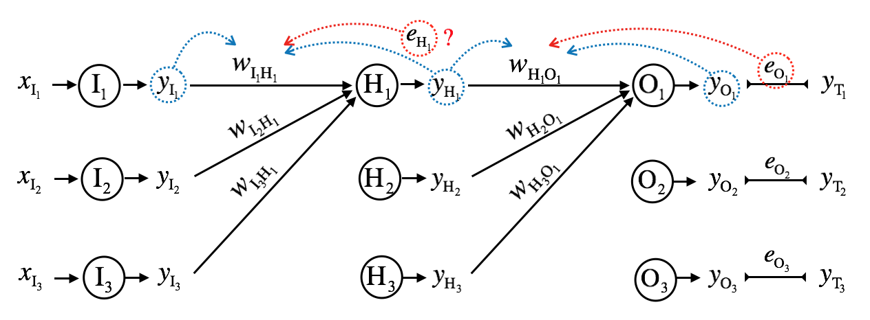
One solution is to think as if \(\mathbf{e_H}^{(i)}\) is generated by \(\mathbf{e_O}^{(i)}\), and this technique is called error backpropagation.
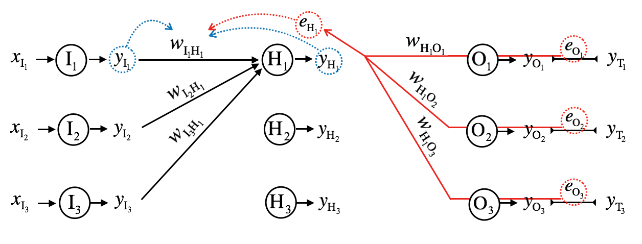
\[e_{H_1} = e_{O_1}{w_{H_1O_1}} + e_{O_2}{w_{H_1O_2}} + e_{O_3}{w_{H_1O_3}}\]
\[e_{H_j} = \sum_{k=1}^{K} w_{H_jO_k}e_{O_k}\]
Thus, in matrix form,
\[\mathbf{e_H} = \begin{bmatrix} e_{H_1} \\ e_{H_2} \\ e_{H_3} \end{bmatrix} % = \begin{bmatrix} w_{H_1O_1} & w_{H_1O_2} & w_{H_1O_3} \\ w_{H_2O_1} & w_{H_2O_2} & w_{H_2O_3} \\ w_{H_3O_1} & w_{H_3O_2} & w_{H_3O_3} \end{bmatrix} % \begin{bmatrix} e_{O_1} \\ e_{O_2} \\ e_{O_3} \end{bmatrix} % = \mathbf{W_{HO}^T}\mathbf{e_O}\]
Note that the transpose of output layer's weight matrix is used. Putting it all together, updating the weights of the hidden layer is as follows:
\[\mathbf{W_{IH}^{(i+1)}} = \mathbf{W_{IH}^{(i)}} + \Delta \mathbf{W_{IH}^{(i)}}\]
\[\Delta \mathbf{W_{IH}^{(i)}} = \alpha \mathbf{e_{H}^{(i)}} \mathbf{y_{H}^{(i)}} \mathbf{(1 - y_{H}^{(i)})} \mathbf{x_{I}^{(i)T}}\]
\[\mathbf{e_{H}^{(i)}} = \mathbf{W_{HO}^{(i)T}} \mathbf{e_{O}^{(i)}}\]
We now know how gradient descent updates the weights of neural network. Let’s wrap it up with an example.
Example
We’ll create a three-layer neural network where the input layer has three nodes, the hidden and output layers each have two nodes. We’ll use sigmoid activation for the hidden and output layers and MSE loss. Let’s set some arbitrary values to the input and output vectors, and weights of each layer.
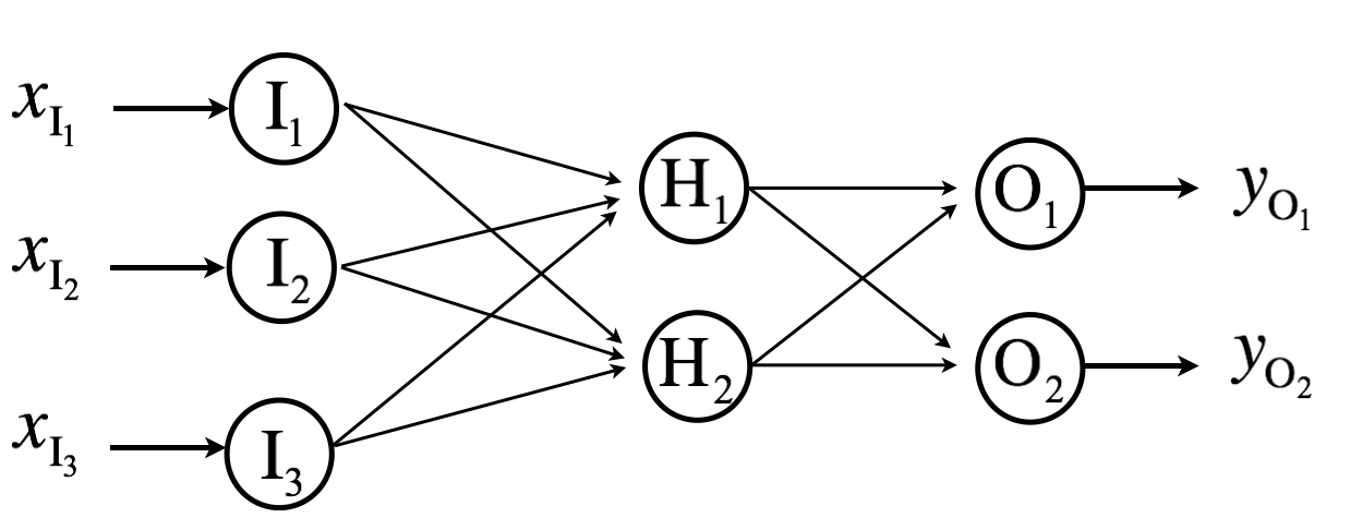
\[\mathbf{x_I} = \begin{bmatrix} x_{I_1} \\ x_{I_2} \\ x_{I_3} \end{bmatrix} % = \begin{bmatrix} 1 \\ 0.5 \\ 0.5 \end{bmatrix} % , \mathbf{y_T} = \begin{bmatrix} y_{T_1} \\ y_{T_2} \end{bmatrix} % = \begin{bmatrix} 1 \\ 1 \end{bmatrix}\]
\[\mathbf{W_{IH}^{(0)}} = \begin{bmatrix} w_{I_1H_1} & w_{I_2H_1} & w_{I_3H_1} \\ w_{I_1H_2} & w_{I_2H_2} & w_{I_3H_2} \end{bmatrix} % = \begin{bmatrix} 1 & 2 & 1 \\ 1 & 1 & 1 \end{bmatrix}\]
\[\mathbf{W_{HO}^{(0)}} = \begin{bmatrix} w_{H_1O_1} & w_{H_2O_1} \\ w_{H_1O_2} & w_{H_2O_2} \end{bmatrix} % = \begin{bmatrix} 1 & -1 \\ -1 & 1 \end{bmatrix}\]
The initial output and loss are as follows:
\[\mathbf{\Sigma_{H}^{(0)}} = \mathbf{W_{IH}^{(0)}x_I} = \begin{bmatrix} 1 & 2 & 1 \\ 1 & 1 & 1 \end{bmatrix} % \begin{bmatrix} 1 \\ 0.5 \\ 0.5 \end{bmatrix} % = \begin{bmatrix} 2.5 \\ 2 \end{bmatrix}\]
\[\mathbf{x_{H}^{(0)}} := \mathbf{y_{H}^{(0)}} = \mathbf{\sigma(\Sigma_H^{(0)})} % = \begin{bmatrix} \frac{1}{1+e^{-2.5}} \\ \frac{1}{1+e^{-2}} \end{bmatrix} % \approx \begin{bmatrix} 0.9241 \\ 0.8808 \end{bmatrix}\]
\[\mathbf{\Sigma_{O}^{(0)}} = \mathbf{W_{HO}^{(0)}x_H^{(0)}} = \begin{bmatrix} 1 & -1 \\ -1 & 1 \end{bmatrix} % \begin{bmatrix} 0.9241 \\ 0.8808 \end{bmatrix} % \approx \begin{bmatrix} 0.0433 \\ -0.0433 \end{bmatrix}\]
\[\mathbf{y_O^{(0)}} = \mathbf{\sigma(\Sigma_O^{(0)})} = \begin{bmatrix} \frac{1}{1+e^{-0.0433}} \\ \frac{1}{1+e^{0.0433}} \end{bmatrix} % \approx \begin{bmatrix} 0.4892 \\ 0.5108 \end{bmatrix}\]
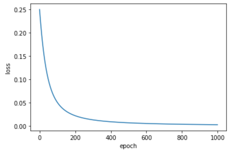
\[MSE^{(0)} = \frac{0.4892^2 + 0.5108^2}{2} \approx 0.2501\]
Let \(\alpha = 0.1\), then
\[\begin{aligned} \mathbf{\Delta W_{HO}^{(0)}} &= \alpha \mathbf{e_{O}^{(0)}} \mathbf{y_{O}^{(0)}} (\mathbf{1} - \mathbf{y_{O}^{(0)}}) \mathbf{y_H^{(0)}} \\ &= 0.1 % \begin{bmatrix} 0.4982 \\ 0.5108 \end{bmatrix} % \begin{bmatrix} 0.5108 \\ 0.4982 \end{bmatrix} % \begin{bmatrix} 1-0.5108 \\ 1-0.4982 \end{bmatrix} % \begin{bmatrix} 0.9241 \\ 0.8808 \end{bmatrix} % = \begin{bmatrix} 0.0113 & 0.0108 \\ 0.0118 & 0.0112 \end{bmatrix} \end{aligned} \]
Finally, the updated weights of the output layer are:
\[\begin{aligned} \mathbf{W_{HO}^{(1)}} &= \mathbf{W_{HO}^{(0)}} + \mathbf{\Delta W_{HO}^{(0)}} \\ &= \begin{bmatrix} 1 & -1 \\ -1 & 1 \end{bmatrix} % + \begin{bmatrix} 0.0113 & 0.0108 \\ 0.0118 & 0.0112 \end{bmatrix} % = \begin{bmatrix} 1.0113 & -0.9892 \\ -0.9882 & 1.0112 \end{bmatrix} \end{aligned}\]
Let's now update the weights of the hidden layer:
\[\begin{aligned} \mathbf{e_H^{(0)}} &= \mathbf{W_{HO}^{(0)}} \mathbf{e_O^{(0)}} \\ &= \begin{bmatrix} 1 & -1 \\ -1 & 1 \end{bmatrix} % \begin{bmatrix} 0.4892 \\ 0.5108 \end{bmatrix} % = \begin{bmatrix} -0.0216 \\ 0.0216 \end{bmatrix} \end{aligned}\]
\[\begin{aligned} \mathbf{\Delta W_{IH}^{(0)}} &= \alpha \mathbf{e_{H}^{(0)}} \mathbf{y_{H}^{(0)}} (1 - \mathbf{y_{H}^{(0)}}) \mathbf{x_I^{(0)T}} \\ &= 0.1 \begin{bmatrix} -0.0216 \\ 0.0216 \end{bmatrix} % \begin{bmatrix} 0.9241 \\ 0.8808 \end{bmatrix} % \begin{bmatrix} 1-0.9241 \\ 1-0.8808 \end{bmatrix} % \begin{bmatrix} 1 & 0.5 & 0.5 \end{bmatrix} \\ &\approx \begin{bmatrix} -0.0002 & -0.0001 & -0.0001 \\ 0.0002 & 0.0001 & 0.0001 \end{bmatrix} \end{aligned}\]
\[\begin{aligned} \mathbf{W_{IH}^{(1)}} &= \mathbf{W_{IH}^{(0)}} + \mathbf{\Delta W_{IH}^{(0)}} \\ &= \begin{bmatrix} 1 & 2 & 1 \\ 1 & 1 & 1 \end{bmatrix} % + \begin{bmatrix} -0.0002 & -0.0001 & -0.0001 \\ 0.0002 & 0.0001 & 0.0001 \end{bmatrix} \\ &\approx \begin{bmatrix} 0.9998 & 1.9999 & 0.9999 \\ 1.0002 & 1.0001 & 1.0001 \end{bmatrix} \end{aligned}\]
Now that we have updated the weights, let’s re-calculate the loss using the same data point (in practice, training data used to update weights should not be used for validation).
Weights and loss before:
\[\mathbf{W_{IH}^{(0)}} = \begin{bmatrix} 1 & 2 & 1 \\ 1 & 1 & 1 \end{bmatrix} , \mathbf{W_{HO}^{(0)}} = \begin{bmatrix} 1 & -1 \\ -1 & 1 \end{bmatrix} , MSE = 0.2501\]
\[\mathbf{W_{IH}^{(0)}} = \begin{bmatrix} 0.9998 & 1.9999 & 0.9999 \\ 1.0002 & 1.0001 & 1.0001 \end{bmatrix} , \mathbf{W_{HO}^{(0)}} = \begin{bmatrix} 1.0113 & -0.9892 \\ -0.9892 & 1.0112 \end{bmatrix}\]
\[\mathbf{\Sigma_H^{(1)}} = \mathbf{W_{IH}^{(1)}}\mathbf{x_I^{(1)}} % = \begin{bmatrix} 0.9998 & 1.9999 & 0.9999 \\ 1.0002 & 1.0001 & 1.0001 \end{bmatrix} % \begin{bmatrix} 1 \\ 0.5 \\ 0.5 \end{bmatrix} % = % \begin{bmatrix} 2.4997 \\ 2.0003 \end{bmatrix}\]
\[\mathbf{y_H^{(1)}} = \mathbf{\sigma(\Sigma_H^{(1)})} = \begin{bmatrix} 0.9241 \\ 0.8808 \end{bmatrix}\]
\[\mathbf{\Sigma_O^{(1)}} = \mathbf{W_{HO}^{(1)}}\mathbf{y_H^{(1)}} % = \begin{bmatrix} 1.0113 & -0.9892 \\ -0.9892 & 1.0112 \end{bmatrix} % \begin{bmatrix} 0.9241 \\ 0.8808 \end{bmatrix} % = % \begin{bmatrix} 0.0630 \\ -0.0221 \end{bmatrix}\]
\[\mathbf{y_O^{(1)}} = \mathbf{\sigma(\Sigma_O^{(1)})} = \begin{bmatrix} 0.5157 \\ 0.4945 \end{bmatrix}\]
\[\mathbf{e_O^{(1)}} = \begin{bmatrix} 1-0.5157 \\ 1-0.4945 \end{bmatrix} % = \begin{bmatrix} 0.4843 \\ 0.5055 \end{bmatrix}\]
\[MSE^{(1)} = \frac{0.4843^2 + 0.50556^2}{2} = 0.2450\]
The loss has reduced!
            import numpy as np

            def initialize_W():
                W_IH = np.array([[1.0, 2.0, 1.0],
                                 [1.0, 1.0, 1.0]])
                W_HO = np.array([[1.0, -1.0],
                                 [-1.0, 1.0]])
                return W_IH, W_HO

            def sigmoid_activation(s):
                y = 1 / (1 + np.exp(-s))
                return y

            def get_y(x, W):
                S = np.dot(W, x)
                y = sigmoid_activation(S)
                return y

            def get_e_O(y_T, y_O):
                e_O = y_T - y_O
                return e_O

            def get_e_H(W_HO, e_O):
                e_H = np.dot(W_HO.T, e_O)
                return e_H

            def get_MSE(e_O):
                MSE = np.sum(e_O ** 2) / e_O.shape[0]
                return MSE

            def update_W(W, alpha, e, y, x):
                delta_W = np.dot((alpha*e*y*(1-y)), x.T)
                W = W + delta_W
                return W

            def train_NN(alpha, epochs):
                for i in range(epochs):
                    if i == 0:
                        W_IH, W_HO = initialize_W()
                        y_H = get_y(x_I, W_IH)
                        y_O = get_y(y_H, W_HO)
                        e_O = get_e_O(y_T, y_O)
                        e_H  = get_e_H(W_HO, e_O)
                        MSE = get_MSE(e_O)
                        print("epoch: ", i, "MSE: ", MSE)
                    else:
                        W_HO = update_W(W_HO, alpha, e_O, y_O, y_H)
                        W_IH = update_W(W_IH, alpha, e_H, y_H, x_I)
                        y_H = get_y(x_I, W_IH)
                        y_O = get_y(y_H, W_HO)
                        e_O = get_e_O(y_T, y_O)
                        e_H = get_e_H(W_HO, e_O)
                        MSE = get_MSE(e_O)
                        print("epoch: ", i, "MSE: ", MSE)

            x_I = np.array([[1.0, 0.5, 0.5]]).T # column vector
            y_T = np.array([[1.0, 1.0]]).T # column vector

            lr = 0.1
            epochs = 1000
            train_NN(alpha=lr, epochs=epochs)