Bayesian Inference
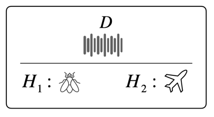
Suppose that you hear an extremely loud (1000 db) noise in a room and want to know what causes the noise. You formulate many hypotheses and use probabilistic approaches to find the hypothesis that can best describe the cause of the noise. Let the noise be data \(D\) and hypothesis be \(H\). There are two approaches; the first approach is to find \(H\) that maximizes \(P(D|H)\), and the second approach is to find \(H\) that maximizes \(P(H|D)\). Both approaches view the conditional probabilities \(P(D|H)\) and \(P(H|D)\) as functions of \(H\), but the two approaches are fundamentally different. The first approach seeks the hypothesis that can best explain the data, while the second approach seeks the hypothesis that is most probable given the data. Which approach do you prefer to use? Confusing? Let’s make the problem simpler. Suppose you have only two hypotheses \(H_1\) and \(H_2\). \(H_1\): there is a fly in the room. \(H_2\): there is an airplane in the room.
\[P(D|H_1) \ \text{vs} \ P(D|H_2)\]
or
\[P(H_1|D) \ \text{vs} \ P(H_2|D)\]
If you chose an approach to compare \(P(D|H_1)\) and \(P(D|H_2)\), you could be a frequentist. If you chose an approach to compare \(P(H_1|D)\) and \(P(H_2|D)\), you could be a Bayesian. Which approach do you prefer to use? Still confusing?
Bayes' Theorem
The conditional probability of an event \(B\), given that an event \(A\) has occurred (that is \(P(A)>0\)), is defined as follows:
\[P(B|A) = \frac{P(A \cap B)}{P(A)} = \frac{P(A,B)}{P(A)}\]
Using that \(P(A,B) = P(A|B)P(B) = P(B|A)P(A)\), Bayes’ theorem describes the relationship between two conditional probabilities \(P(A|B)\) and \(P(B|A)\) as follows:
\[P(B|A) = \frac{P(A|B)P(B)}{P(A)}\]
Now, we will modify the above equation slightly. For \(K \in \mathbb{Z}^+\), let the sets \(B_1, B_2, ..., B_K\) be such that \(S = \bigcup_{k=1}^{K} B_{k}\) and \(B_i \bigcap B_j = \emptyset\) for \(i \ne j\).
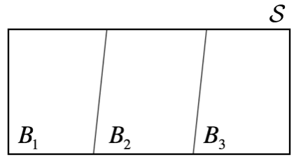
Then, the collection of sets \(\{B_1, B_2, ..., B_K \}\) is said to be a partition of \(S\). If event \(A\) occurs as any subset of \(S\), set \(A\) can be decomposed as follows:
\[A = (A \cap B_1) \cup (A \cap B_2) \cup ... \cup (A \cap B_K)\]
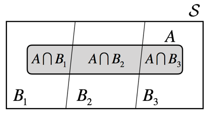
Then, it is easy to see \(P(A)\) can be expressed as follows:
\[\begin{equation} \begin{aligned} P(A) &= \sum_{k=1}^K P(A \cup B_k) = \sum_{k=1}^K P(A, B_k) \\ &= \sum_{k=1}^K P(A|B_k)P(B_k) \end{aligned} \end{equation}\]
Now, we can write Bayes' theorem as follows:
\[P(B_k|A) = \frac{P(A|B_k)P(B_k)}{\sum_{k=1}^K P(A|B_k^{'})P(B_k^{'})}\]
Note that the denominator in right hand side is a normalizing constant such that \(\sum_k P(B_k|A)=1\) (for example, \(\frac{a}{(a+b+c)} + \frac{b}{(a+b+c)} + \frac{c}{(a+b+c)} = 1\)).
This simple theorem exhibits its power in computational biology, artificial intelligence, finance, and even in astrophysics. A well known easy example is to calculate the probability of disease given that diagnostic test shows positive result, that is \(P(1|+)\).
Let 1 (diseased) and 0 (healthy) denote the health state of a person, and let + and - denote the result of diagnostic test. Then, \(P(1)\) represents the prevalence rate of a particular disease that is the target of diagnosis. We assume that the prevalence rate is known to us: \(P(1)=0.00001\). Suppose that a company developed a diagnostic kit for this disease. The company examined 1,000 diseased people and 1,000 healthy people using the kit to evaluate the kit’s performance and observed that 999 diseased people got positive result and 1 healthy person also got positive results. Thus, \(P(+|1)\) estimated by the true positive rate (TPR) is 0.999 and \(P(+|0)\) estimated by the false positive rate (FPR) is 0.001. If you are diagnosed as positive, what will be the probability that you are actually diseased? Note that \(P(+|1)\) and \(P(+|0)\) do not directly tell you the probability you want. These probabilities are about the kit’s performance not your health state. What you want to know is \(P(1|+)\) not \(P(+|1)\). Let’s use Bayes’ theorem to calculate \(P(1|+)\).
\[\begin{equation} \begin{aligned} P(1|+) &= \frac{P(+|1)P(1)}{P(+|1)P(1) + P(+|0)P(0)} \\ &= \frac{0.999 \times 0.00001}{0.999 \times 0.00001 + 0.001 \times 0.99999} \\ \approx 0.0099 \end{aligned} \end{equation}\]
The probability of disease is only 0.0099 even if diagnosed as positive! Why? Such result is because the kit’s performance is not satisfactory (TPR is very low and FRP is very high) compared to low prevalence rate of the disease. Above example is very good to spark people’s interest in Bayesian inference, but there is an important point many people miss. Before you are examined, your probability of disease was \(P(1)=0.00001\). But when you have a positive diagnostic result, this probability is updated to \(P(1|+) \approx 0.0099\). It is almost \(\times 1,000\) increase!
Prior, Likelihood and Posterior
Let's revisit the problem mentioned in introduction and re-write the Bayes' theorem as follows:
\[P(H_k|D) = \frac{P(D|H_k)P(H_k)}{\sum_{k=1}^K P(D|H_k)P(H_k)}\]
First note that denominator is normalizing constant (it is called marginal likelihood). Thus, above equation can be written as follows:
\[P(H_k|D) \propto P(D|H_k)P(H_k)\]
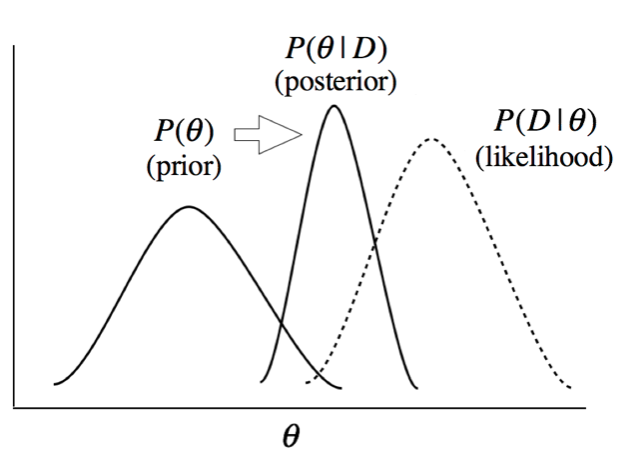
The term \(P(H_k)\) is called prior distribution of simply prior. As mentioned in disease example, prior describes probability distribution before we see the data. \(P(H_k|D)\) is called posterior distribution. After seeing the data, prior is updated to posterior. During the update, the likelihood, \(P(D|H_k)\), is used. Interpretation of likelihood is a bit complicated. The likelihood is the probability of data assuming that the condition is true.
Now, think of the the problem mentioned in introduction section. Comparing \(P(D|H_1)\) and \(P(D|H_2)\) is to find the hypothesis that results in larger likelihood. Which likelihood is larger? Be careful that this question does not ask which hypothesis is true or not. \(P(D|H_2)\) is higher than \(P(D|H_1)\). A fly in a room cannot generate such a loud noise. If there is an airplane in your room, it is highly likely to hear 1000 db noise. Again, the question did not ask whether an airplane is in your room or not. The question asked "if there is an airplane in your room" how much likely are you to hear the loud noise. Actually, this question/answer is not about what we want to know. What we want to know was, given that you hear a loud noise, what is the probability of there being a fly/airplane in your room, which requires the comparison of two posteriors, \(P(H_1|D)\) and \(P(H_2|D)\).
Frequentist's methods of inference are mainly based on likelihood, while Bayesian methods are mainly based on posterior. Many probabilistic and statistical methods commonly used (e.g., t-test, ANOVA, regression, p-value, confidence interval) are all frequentist's methods. The weakness (in a sense of frequentists) of Bayesian approach is that it requires prior in addition to data to draw posterior, and there is no concrete rule for selecting prior. Bayesians think probability is a subjective belief, thus no one can make arguments against other's priors as their beliefs. Because likelihood deals with only data (no room for subjectivity), frequentists methods had been viewed as objective and widely used. Another reason the Bayesian approach did not prevail in the past is that it requires complex, intractable integrations to calculate the marginal likelihood. However, with the development of computational tools (hardwares and numerical algorithms such as Markov chain Monte Carlo sampling), Bayesian approaches are getting more attentions. In the following sections, I will introduce one of the widely used frequentist method of parameter estimation, maximum likelihood estimation, then discuss Bayesian method of estimation.
Maximum Likelihood Estimation
Maximum likelihood estimation/estimate (MLE) is simply expressed as follows:
\[\hat{\theta}^{ML} = \text{argmax}_{\theta} P(D|\theta)\]
Since \(P(D|\theta)\) is viewed as a function of \(\theta\) in the likelihood-based method, we need to define the likelihood function as \(L(\theta) := P(D|\theta)\). Then, it becomes an optimization problem, which can be solved by differentiation if \(L(\theta)\) is a monotonic function. And because \(P(D|\theta)\) is often in a form of joint probability of IID RVs (e.g., \(P(y_1, y_2, ..., y_n | \theta) = P(y_1|\theta)P(y_2|\theta)...P(y_n|\theta)\), we use log likelihood to make differentiation easier. Practically, MLE can be obtained as follows:
\[\frac{d}{d\theta}\text{log} L(\theta) \biggr\rvert_{\theta = \hat{\theta}^{ML}} = 0\]
Let’s estimate the parameter of binomial distribution \(\theta_H\). Suppose \(n\) coin-tosses results in observations \(D = \mathbf{y} = [y_H, y_T]\), where \(y_H\) is the number of heads observed and \(y_T\) is the number of tails observed.
\[\begin{equation} \begin{aligned} L(\theta_H) &= M(\mathbf{y})\theta_H^{y_H}(1-\theta_H)^{y_T} \\ \text{log}L(\theta_H) &= \text{log}M(\mathbf{y}) + \text{log}\theta_H^{y_H} + \text{log}(1-\theta_H)^{y_T}\\ &= \text{log}M(\mathbf{y}) + y_H\text{log}\theta_H + y_T\text{log}(1-\theta_H) \end{aligned} \end{equation}\]
\[\frac{d}{d\theta_H}\text{log}L(\theta) = y_H(\frac{1}{\theta_H}) + y_t(-\frac{1}{1-\theta_H})\]
\[\implies y_H (\frac{1}{\hat{\theta_H}^{ML}}) + y_T(-\frac{1}{1 - \hat{\theta_H}^{ML}}) = 0\]
\[\implies \hat{\theta_H}^{ML} = \frac{y_H}{y_H + y_T} = \frac{y_H}{n}\]
Result indicates that \(\hat{\theta_H}^{ML}\) is consistent with frequentist’s definition of probability. Similarly, MLE of multinomial distribution is \(\hat{\theta_k}^{ML} = \frac{y_k}{n}\).
Bayesian Estimation
It would be best to mention here that the concept of parameter is also different between frequentists and Bayesians. In frequentist’s approach, \(\theta\) is unknown but a fixed value (hence no direct probabilistic statement about the parameter is possible; p-values or confidence intervals are all about the data not the parameter). In Bayesian approach, \(\theta\) is unknown but a random variable (hence direct probabilistic statement about parameter is possible). Thus, Bayesian inference is always made using probability distributions of \(\theta\).
\[P(\theta|D) = \frac{P(D|\theta)P(\theta)}{\int_\theta P(D|\theta)P(\theta) d\theta} \propto P(D|\theta)P(\theta)\]
Bayesian inference begins with setting a prior distribution before we see the data. Although the prior can be a subjective belief, it would be good to reflect our prior knowledge about the parameter. As shown in this this article describing beta and Dirichlet distributions, our prior belief about target parameter can be expressed using parameters of prior distribution, which is called hyperparameters. If we don’t have ant information about the prior, we can use uniform distribution for the prior distribution (uniform prior is often called a ’flat’ prior). Multiplied by likelihood, prior distribution is then update to posterior.
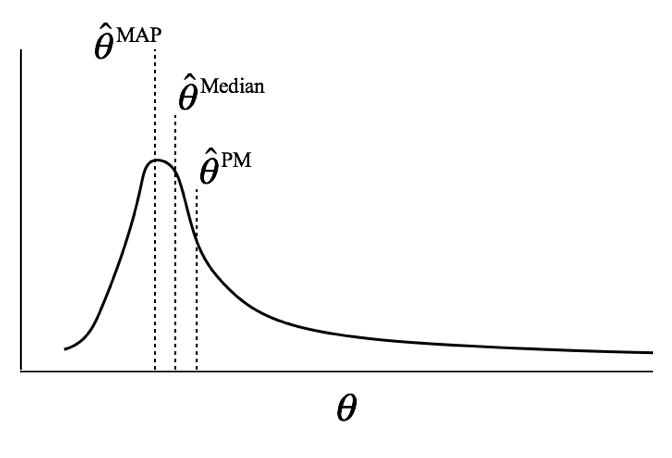
Bayesian inference is always made using posterior probability distribution of \(\theta\), and parameter estimation is carried out by summarizing the posterior distribution. There are three commonly used methods for summarizing probability distribution: expected value, median, and mode (maximum density); these can also be used to summarize the posterior distribution.
Posterior mean (PM) is Bayesian parameter estimate that summarizes the posterior distribution using the expected value.
\[\hat{\theta}^{PM} = E(\theta|D) = \int_\theta \theta P(\theta|D)d\theta\]
Maximum a posteriori (MAP) finds parameter value that has the highest density (mode).
\[\hat{\theta}^{MP} = \text{argmax}_{\theta}P(\theta|D) = \text{argmax}_{\theta}P(D|\theta)P(\theta)\]
Posterior median summarizes the posterior distribution using the median.
\[\hat{\theta}^{Posterior Median} = \int_{-\infty}^{median} P(\theta|D)d\theta = 0.5\]
Each estimate has pros and cons, and choice of estimate could depend on the expected shape of posterior. If the posterior has a long tail (highly skewed), MAP could be a better choice than PM.
Conjugate Priors
Finding the posterior distribution is not easy because the product of prior and likelihood can be a complex function and marginal likelihood requires integration of the complex function. Moreover, calculation of PM requires additional integration.
\[\hat{\theta}^{PM} = \int_{\theta}\theta \frac{P(D|\theta)P(\theta)}{\int_{\theta}P(D|\theta)P(\theta) d\theta} d\theta\]
If parameter dimensionality is high, then multiple multi-dimensional integration is required and analytic solution is virtually impossible. One solution is to use MCMC sampling. But there are some probability distributions for priors, which does not require integrations to find posterior. These distributions are called conjugate priors. Let’s look at two of them with examples.
Binomial Likelihood and Beta Prior
To make equations more readable, binomial likelihood is denoted by \(Binom(\mathbf{y}|\theta)\), where \(\mathbf{y} = [y_H, y_T]\) and \(\theta = \theta_H\), and beta PDF for prior is denoted by \(Beta(\theta|\mathbf{\alpha})\), where \(\mathbf{\alpha} = [\alpha_H, \alpha_T]\). Also \(M(\mathbf{y})\) denotes binomial coefficient and \(B(\mathbf{\alpha})\) denotes beta function.
\[\begin{equation} \begin{aligned} P(\theta|\mathbf{y}) &= \frac{Binom(\mathbf{y}|\theta)Beta(\theta|\mathbf{\alpha})}{\int_0^1 Binom(\mathbf{y}|\theta)Beta(\theta|\mathbf{\alpha}) d \theta} \\ &= \frac{M(\mathbf{y})\theta^{y_H}(1-\theta)^{y_T} B(\mathbf{\alpha})^{-1}\theta^{\alpha_H -1}(1-\theta)^{\alpha_T -1}}{\int_0^1 M(\mathbf{y})\theta^{y_H}(1-\theta)^{y_T} B(\mathbf{\alpha})^{-1}\theta^{\alpha_H -1}(1-\theta)^{\alpha_T -1} d\theta} \\ &= \frac{\theta^{y_H}(1-\theta)^{y_T} \theta^{\alpha_H -1}(1-\theta)^{\alpha_T -1}}{\int_0^1 \theta^{y_H}(1-\theta)^{y_T} \theta^{\alpha_H -1}(1-\theta)^{\alpha_T -1} d\theta} \\ &= \frac{\theta^{(\alpha_H + y_H)-1} (1-\theta)^{(\alpha_T + y_T)-1}}{\int_0^1 \theta^{(\alpha_H + y_H)-1} (1-\theta)^{(\alpha_T + y_T)-1} d\theta} \\ &= \frac{\theta^{(\alpha_H + y_H)-1} (1-\theta)^{(\alpha_T + y_T)-1}}{B([\alpha_H + y_H], [\alpha_T + y_T])} \\ &= Beta(\theta|\mathbf{\alpha} + \mathbf{y}) \end{aligned} \end{equation}\]
Posterior is \(Beta(\theta|\mathbf{\alpha} + \mathbf{y})\), which means prior \(Beta(\theta|\mathbf{\alpha})\) is updated to posterior by incorporating the data \(\mathbf{y}\) into its parameters. Because the formula to calculate the expected value of beta distribution is already known as \(E[\theta|\alpha_1, \alpha_2] = \frac{\alpha_1}{\alpha_1 + \alpha_2}\), we can simply calculate the posterior mean as follows:
If we believe that the coin is balanced (\(E(\theta)=0.5\)) before observing the result of the coin-toss experiment, we can set \(\alpha_H = \alpha_T = 5\) for the hyperparameters of the prior distribution. Then, after observing the data, say \(y_H =3\) and \(y_T =7\), our prior is updated to \(E(\theta|\mathbf{y})=0.4\). If we have a very strong prior (belief) that coin is skewed (e.g., \(\alpha_H =1\) and \(\alpha_T =999\)), weak data (e.g., \(y_H = y_T = 5\)) have only a small effect on the update. In this case PM will be \(E(\theta|\mathbf{y})\approx 0.006\). If we have a weak prior compared to data, data will dominate the posterior. If we have no prior information about \(\theta\), our ignorance can be expressed by Jeffrey’s beta prior (\(Beta(\theta|\alpha_1 = \alpha_2 = 0.5)\) or uniform prior, which is \(Beta(\theta|\alpha_1 = \alpha_2 = 1)\).
Multinomial likelihood and Dirichlet prior
Multinomial likelihood is denoted by \(Multinom(\mathbf{y}|\mathbf{\theta})\) and Dirichlet prior is denoted by \(Dir(\mathbf{\theta}|\mathbf{\alpha})\). Multi-dimensional integration is not explicitly represented.
\[\begin{equation} \begin{aligned} P(\mathbf{\theta}|\mathbf{y}) &= \frac{Multinom(\mathbf{y}|\mathbf{\theta})Dir(\mathbf{\theta}|\mathbf{\alpha})}{\int_\theta Multinom(\mathbf{y}|\mathbf{\theta})Dir(\mathbf{\theta}|\mathbf{\alpha}) d \mathbf{\theta}} \\ &= \frac{M(\mathbf{y}) \prod_{k=1}^K \theta_k^{y_k} Z(\mathbf{\alpha})^{-1}\prod_{k=1}^K \theta_k^{\alpha_k-1}}{\int_\theta M(\mathbf{y}) \prod_{k=1}^K \theta_k^{y_k} Z(\mathbf{\alpha})^{-1}\prod_{k=1}^K \theta_k^{\alpha_k-1} d \mathbf{\theta}}\\ &= \frac{ \prod_{k=1}^K \theta_k^{y_k} \prod_{k=1}^K \theta_k^{\alpha_k-1}}{\int_\theta \prod_{k=1}^K \theta_k^{y_k} \prod_{k=1}^K \theta_k^{\alpha_k-1} d \mathbf{\theta}} \\ &= \frac{\prod_{k=1}^K \theta_k^{(\alpha_k + y_k)-1}}{\int_\theta \prod_{k=1}^K \theta_k^{(\alpha_k + y_k)-1} d \mathbf{\theta}} \\ &= \frac{\prod_{k=1}^K \theta_k^{(\alpha_k + y_k)-1}}{Z(\mathbf{\alpha} + \mathbf{y})}\\ &= Dir(\mathbf{\theta}|\mathbf{\alpha} + \mathbf{y}) \end{aligned} \end{equation}\]
Similar to binomial likelihood and beta prior, Dirichlet prior \(Dir(\mathbf{\theta}|\mathbf{\alpha})\) with multinomial likelihood results in Dirichlet posterior \(Dir(\mathbf{\theta}|\mathbf{\alpha}+\mathbf{y})\). PM is as follows:
\[\hat{\theta_k}^{PM} = \frac{\alpha_k + y_k}{\sum_{k=1}^K (\alpha_k + y_k)} = \frac{\alpha_k + y_k}{\sum_{k^{'}=1}^K \alpha_{k^{'}} + \sum_{k^{'}=1}^K y_{k^{'}}}\]
Considering that Bayesian inference is a process of updating prior (belief), a posterior drawn by observing data becomes the prior for the next time, which is very similar to our brain's learning process. And such update process continues until no more update occurs. Thus, even if we started from a very subjective (or absurd) prior, we will eventually reach an objective posterior. Also, with very big data, both Bayesian approach and frequentist's approach draw the same conclusion, while Bayesian approach is especially useful for small or limited data.
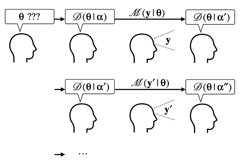
As shown in above diagram, the hyperparameters of prior (e.g., Dirichlet parameter ) plays a crucial role in the Bayesian update. Thus, how to set the hyperparameter is very important in Bayesian inference.
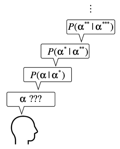
Considering that parameters are random variables in Bayesian inference, we can have a prior distribution of hyperparameter \(\mathbf{\alpha}\), a prior distribution of hyperparameter \(\mathbf{\alpha^*}\), and so on. This topic is related to the estimation of prior, which I will discuss later.