Multinomial Distribution and Dirichlet Distribution
Mathematical models can be classified into deterministic model and probabilistic model, and probabilistic model tells us the probability of outcomes in the form of probability distribution. For example, we can calculate the probability of observing three heads in ten coin-toss trials using probability mass function (PMF) of binomial distribution. While there are many probability distributions used to model real phenomena, I will describe two distributions which are useful for explaining Bayesian inferences. I will begin with Bernoulli trial.
Bernoulli trial is a experiment with two outcomes. If we model a single coin-toss using Bernoulli trial, the domain of Bernoulli random variable is \(\mathscr{X} = \{0,1\} = \{Head, Tail\}\).
\[X= \left\{ \begin{array}{ll} 1, \text{with probability } \theta_H \\ 0, \text{with probability } \theta_T = (1-\theta_H) \\ \end{array} \right.\]
Binomial Distribution
Suppose we repeated 3 independent coin-toss experiment and recorded outcomes sequentially.
\[Data^{'} = HHT\]
Given the parameter \(\theta_H (\theta_T = 1-\theta_H)\), the probability of observing the data is
\[P(Data^{'} = \theta_H, \theta_T) = \theta_H \theta_H \theta_T = \theta_H^2 \theta_T\]
Now, let’s say we flip a coin three times and got two heads and one tail.
\[Data = [2 Hs, 1 T] =\{HHT, HTH, THH\}\]
Since
\[P(Data^{'}_1 | \theta_H, \theta_T) = P(HHT|\theta_H, \theta_T) = \theta_H \theta_H \theta_T = \theta_H^2 \theta_T\]
\[P(Data^{'}_2 | \theta_H, \theta_T) = P(HTH|\theta_H, \theta_T) = \theta_H \theta_T \theta_H = \theta_H^2 \theta_T\]
\[P(Data^{'}_2 | \theta_H, \theta_T) = P(THH|\theta_H, \theta_T) = \theta_T \theta_H \theta_H = \theta_H^2 \theta_T\]
\(P(Data|\theta_H,\theta_T)\)is simply \(\theta_H^2\theta_T\) multiplied by the number of ways of 2 Hs and 1 T occur, which can be calculated using binomial coefficient.
\[\begin{equation} \begin{aligned} P(Data|\theta_H, \theta_T) &= P(Data^{'}_1|\theta_H, \theta_T) + P(Data^{'}_2|\theta_H, \theta_T) + P(Data^{'}_3|\theta_H, \theta_T) \\ &= {3 \choose 2}\theta_H^2\theta_T = 3\theta_H^2\theta_T \end{aligned} \end{equation}\]
Above description is the macrostate/microstate interpretation of binomial probability. \(Data\) corresponds to the macrostate of the RV and \(Data^{'}\) corresponds to microstate; we will revisit this in Entropy post. Conventionally, binomial distribution is explained by summation of independent and identically distributed (IID) RVs that follow Bernoulli distribution.
\[Y = \sum_{i=1}^n X_i, X_i \sim Bernoulli(\theta_H)\]
Then, \(Y\) is said to follow binomial distribution. The PMF of binomial distribution is represented as follows:
\[p(y|\theta_H) = {n \choose y}\theta_H^y(1-\theta_H)^{n-y} = {n \choose y}\theta_H^y \theta_T^{n-y}, y=0,1,2,...,n\]
Multinomial Distribution
I will modify above binomial PMF with a little abuse of notations. First, I will consider the number of heads (\(y_H\)) and the number of tails (\(y_T\)) separately, and represent the data using a vector \(\mathbf{y} = [y_H,y_T]=[y_1,y_2]\). Similarly, I will use a vector notation for two parameters \(\mathbf{\theta}=[\theta_H,\theta_T]=[\theta_1,\theta_2]\). Although \(y_H\) and \(y_T\) are not independent from each other because \(y_H + y_T = n\) and \(\theta_H\) and \(\theta_T\) are also not independent from each other because \(\theta_H + \theta_T = 1\), vector notations will make the formula simpler.
\[p(\mathbf{y}|\mathbf{\theta}) = \frac{(y_1 + y_2)!}{y_1!y_2!}\theta_1^{y_1}\theta_2^{y_2} = \frac{(y_1 + y_2)!}{y_1!y_2!}\prod_{k=1}^K \theta_k^{y_k}, K=2\]
Now, consider the case \(K>2\), a die-roll experiment for example (\(K=6\)). And recall that binomial coefficient is a special case of multinomial coefficient \(M(\mathbf{y})\). Then, for any \(K\ge 2\),
\[p(\mathbf{y}|\mathbf{\theta}) = M(\mathbf{y})\prod_{k=1}^K \theta_k^{y_k} = \frac{(\sum_{k=1}^K y_k)!}{\prod_{k=1}^K y_k!} \prod_{k=1}^K \theta_k^{y_k}\]
This is the PMF of multinomial distribution. For example, the probability of observing 2 As and 2 Ts and 3 Gs and 3 Cs in a DNA sequence of length \(L=10\) is calculated as
\[p(\mathbf{y}|\mathbf{\theta}) = \frac{10!}{2!2!3!3!}\theta_A^2 \theta_T^2 \theta_G^3 \theta_C^3\]
The expected value and variance of multinomial RV is as follows:
\[E(y_k) = [\sum_{k^{'}=1}^K y_k^{'}]\theta_k \equiv n\theta_k\]
\[V(y_k) = [\sum_{k^{'}=1}^K y_k^{'}]\theta_k (1-\theta_k) \equiv n\theta_k (1-\theta_k)\]
Binomial distribution and multinomial distribution are distributions of discrete RVs. In the following two sections, I will discuss two distributions of continuous RVs.
Beta Distribution
The probability distribution of a continuous RV of which domain is \([0,1]\) (from 0 to 1) can be described using beta distribution. Before introducing the beta distribution, I will briefly explain how to convert a general function to PDF.
Let \(g(y)\) be the general function, and suppose we want to convert \(g(y)\) to PDF \(f(y)\). First integrate \(g(y)\) to get normalizing constant \(I\).
\[I = \int_{y \in Y} g(y)dy\]
Then we can obtain
\[f(y) = \frac{g(y)}{I}\]
The domain of RV \(Y\) should satisfy \(I \ne 0\) and \(f(y) \ge 0\). We can confirm that \(f(y)\) is a proper PDF.
\[\int_{y \in Y}f(y)dy = \int_{y \in Y} \frac{g(y)}{I}dy = \frac{1}{I}\int_{y \in Y} g(y)dy = 1\]
Now, let \(h(x) = x^{\alpha-1}e^{-x}\). Then, we obtain a gamma function.
\[I = \Gamma(\alpha) = \int_0^{\infty} h(x)dx = \int_0^{\infty} x^{\alpha -1}e^{-x}dx\]
Gamma function has interesting property that \(\Gamma(\alpha) = (\alpha-1)\Gamma(\alpha-1)\) and if \(\alpha \in \mathbb{N}\), \(\Gamma(\alpha) = (\alpha-1)\) (gamma function can be used as a normalizing constant to derive PDF of gamma distribution).
Now, let \(g(x) = x^{\alpha -1}(1-x)^{\beta -1}\), which is in part similar to the PMF of binomial distribution. Then, we obtain a beta function, which is a function of gamma functions.
\[\begin{equation} \begin{aligned} I &= B(\alpha , \beta) = \int_0^1 g(x)dx = \int_0^1 x^{\alpha-1}(1-x)^{\beta-1}dx \\ &= \frac{\Gamma(\alpha)\Gamma(\beta)}{\Gamma(\alpha + \beta)} \end{aligned} \end{equation}\]
Finally using the beta function as normalizing constant, we obtain the PDF of beta distribution.
\[f(x|\alpha , \beta) = \frac{g(x)}{B(\alpha , \beta)} = \frac{x^{\alpha -1}(1-x)^{\beta -1}}{[\frac{\Gamma(\alpha)\Gamma(\beta)}{\Gamma(\alpha + \beta)}]}\]
At this point, by recalling \(0 \le x \le 1\), I replace \(x\) with \(\theta\).
\[f(\theta|\alpha ,\beta) = \frac{\theta^{\alpha -1}(1-\theta)^{\beta -1}}{[\frac{\Gamma(\alpha)\Gamma(\beta)}{\Gamma(\alpha + \beta)}]}, 0 \le \theta \le 1\]
And with a little abuse of notations: \(\mathbf{\theta} := [\theta_1, \theta_2]\), where \(\theta_1 = \theta\) and \(\theta_2 = (1-\theta)\) and \(\mathbf{\alpha}:= [\alpha_1, \alpha_2]\), where \(\alpha_1 = \alpha\) and \(\alpha_2 = \beta\), the beta PDF is expressed as
\[f(\mathbf{\theta}|\mathbf{\alpha}) = \frac{\theta_1^{\alpha_1 -1} \theta_2^{\alpha_2 -1}}{\frac{\Gamma(\alpha_1)\Gamma(\alpha_2)}{\Gamma(\alpha_1 + \alpha_2)}}, \theta_1+\theta_2=1\]
The expected value and variance of RV \(\theta_1 = 1-\theta_2\) is as follows:
\[E(\theta_1|\alpha)=\frac{\alpha_1}{\alpha_1+\alpha_2}\]
\[V(\theta_1|\alpha)=\frac{\alpha_1 \alpha_2}{(\alpha_1+\alpha_2)^2} \times \frac{1}{(\alpha_1+\alpha_2 + 1)}\]
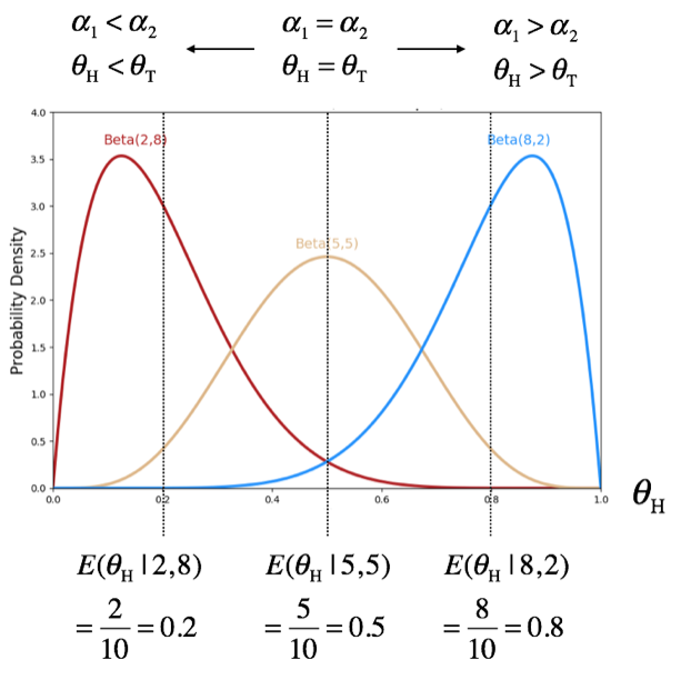
Considering that \(0 \le \theta_i \le 1\) and \(\theta_1 + \theta_2 = 1\), beta distribution can be viewed as a probability distribution of probability. For example, if we think \(\theta_H = \theta_1\) and \(\theta_T = \theta_2\), beta distribution can be used to model the parameter of binomial PDF \(p(\mathbf{y}|\mathbf{\theta})\).
Dirichlet Distribution
Now, I will modify the beta PDF more. First, let's generalize the nominator part of beta PDF to accommodate more than three thetas.
\[\theta_1^{\alpha_1 -1}\theta_2^{\alpha_2 -1}...\theta_K^{\alpha_K -1} = \prod_{k=1}^K \theta_k^{\alpha_K -1}, \sum_{k=1}^K \theta_k =1\]
Second, let's generalize the beta function (normalizing constant in beta PDF) and arbitrarily name it a zeta function.
\[Z(\mathbf{\alpha}) = \frac{\Gamma(\alpha_1)\Gamma(\alpha_2)...\Gamma(\alpha_K)}{\Gamma(\alpha_1 + \alpha_2 + ... + \alpha_K)} = \frac{\prod_{k=1}^K \Gamma(\alpha_k)}{\Gamma(\sum_{k=1}^K \alpha_k)}\]
Then, we get the PDF of Dirichlet distribution.
\[f(\mathbf{\theta}|\mathbf{\alpha}) = \frac{\prod_{k=1}^K \theta_k^{\alpha_k -1}}{Z(\mathbf{\alpha})}, \sum_{k=1}^K \theta_k = 1\]
Thus, beta distribution is the special case (\(K=2\)) of Dirichlet distribution as binomial distribution is a special case of multinomial distribution. Expected value and variance of Dirichlet distribution are also the multivariate versions of the expected value and variance of beta distribution.
\[E(\theta_k|\mathbf{\alpha}) = \frac{\alpha_k}{A}, A=\sum_{k^{'}=1}^K \alpha_{k^{'}=1}\]
\[V(\theta_k|\mathbf{\alpha}) = [\frac{\alpha_k}{A}(1-\frac{\alpha_k}{A})] \times \frac{1}{(A+1)}\]
Remark
You may remember that Bayesian probability is a belief. We can numerically express our belief using the beta distribution. For example, if we believe a coin is balanced, our belief on this coin’s parameter (\(\theta_T = \theta_H\)) can be expressed using two parameters (\(\alpha_T = \alpha_H\)) of beta distribution such that the expected value of beta RV is \(E(\theta_H|\mathbf{\alpha}) = \frac{\alpha_H}{(\alpha_H + \alpha_T)} = 0.5\). If we believe the coin is unbalanced, we can use \(\alpha_T > \alpha_H\) or \(\alpha_T < \alpha_H\). We can also numerically express the strength of our belief. For example, setting \(\alpha_T = \alpha_H = 2\) and setting \(\alpha_T = \alpha_H = 10\) both result in the same expected value but different variances; the higher the \(\alpha\) values the lower the variance. Higher variance of RV results in a sharp peak of PDF curve concentrating densities in a narrower range, which reflects our stronger belief. In the case \(K>2\) (e.g., die roll or DNA/RNA/protein sequences), we can use Dirichlet distribution.
To model phenomena with \(K\) discrete outcomes, we can use multinomial distribution represented by its PMF \(p(\mathbf{y}|\mathbf{\theta})\). In Bayesian sense, this PMF is in a form of conditional probability, which means that we need to know true values of parameters \(\mathbf{\theta}\) before we do modeling. What if we don’t know the exact value of the parameters? We need to get estimates of them (\(\hat{\mathbf{\theta}}\)) and then use the model with the estimates \(p(\mathbf{y}|\hat{\mathbf{\theta}})\). There are basically two approaches to get the estimates of the parameters: frequentist’s and Bayesian approaches. Well-known frequentist’s method is maximum likelihood estimation, which seeks the parameter value that maximize the likelihood, \(p(\mathbf{y}|\hat{\mathbf{\theta}})\) as a function of \(\hat{\mathbf{\theta}}\). Bayesian approach seeks the distribution of parameter using Bayes’ theorem. To estimate the parameter, frequentist approach requires only data, but Bayesian approach require our prior belief on the parameter in addition to data. As mentioned above, our prior belief can be numerically incorporated as Dirichlet distribution. We will discuss parameter estimation later.