Logit and Bayesian Inference
In probability theory, the logit (logistic unit) of probability \(p\) is the logarithm of odds, which is \(\frac{p}{(1-p)}\).
\[\text{logit}(p) = \text{log}\frac{p}{1-p}\]
The inverse of logit function is a logistic (sigmoid) function.
\[p = \sigma(\text{logit}) = \frac{1}{1+e^{-\text{logit}}}\]
If we let \(P(M)\) be the prior probability that something we want to prove is true and let \(P(R)=1-P(M)\). The prior ratio becomes the prior odds.
\[\frac{P(M)}{1-P(M)}=\frac{P(M)}{P(R)}\]
Similarly, the posterior ratio, which is the product of likelihood ratio (LR) and prior ratio (PR), is also in the form of odds. For more details, please refer to this article .
\[\frac{P(M|D)}{1-P(M|D)} = \frac{P(M|D)}{P(R|D)} = \frac{P(D|M)}{P(D|R)} \cdot \frac{P(M)}{P(R)} = LR \cdot PR\]
Note that likelihood ratio cannot be said to be in the form of odds because it is not always true that \(P(D|R) = 1-P(D|M)\). If data is comprised of \(n\) independent features or observations (\(\mathbf{x} = [x_1, x_2, ..., x_n]\)) of an object, the posterior odds is as follows:
\[\frac{P(M|\mathbf{x})}{P(R|\mathbf{x})} = [\prod_{i=1}^n \frac{P(x_i|M)}{P(x_i|R)}]\frac{P(M)}{P(R)}\]
Let’s denote the log posterior odds by logit \(\psi\).
\[\begin{equation} \begin{aligned} \psi &= \text{log}\frac{P(x_1|M)}{P(x_1|R)} + \text{log}\frac{P(x_2|M)}{P(x_2|R)} + ... + \text{log}\frac{P(x_n|M)}{P(x_n|R)} + \text{log}\frac{P(M)}{P(R)} \\ &= [\sum_{i=1}^n \text{log}\frac{P(x_i|M}{P(x_i|R)}]+\text{log}\frac{P(M)}{P(R)} \end{aligned} \end{equation}\]
Now, let’s express posterior probability using the logit \(\psi\).
\[\begin{equation} \begin{aligned} P(M|\mathbf{x}) &= \frac{P(\mathbf{x}|M)P(M)}{P(\mathbf{x}|M)P(M) + P(\mathbf{x}|R)P(R)} \\ &= \frac{1}{\frac{P(\mathbf{x}|M)}{P(\mathbf{x}|R)} \frac{P(M)}{P(R)} + 1} \\ &= \frac{1}{1+ (LR \cdot PR)^{-1}} \\ &= \frac{1}{1+e^{-\text{log}(LR \cdot PR)}} \\ &= \frac{1}{1+ e^{-[\text{log}LR + \text{log}PR]}} \\ &= \frac{1}{1+e^{-\psi}} \end{aligned} \end{equation}\]
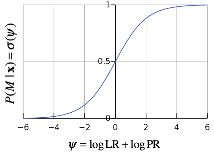
Thus, posterior probability is a sigmoid function of logit \(\psi\). When \(\psi\) is greater than zero, the probability that the model or something we want to prove is true is greater than 0.5.
You may remember the computational biology example (searching viral sequences in eukaryotic genome) from this article . Here I write the key equation.
\[\begin{equation} \begin{aligned} \frac{P(E|\mathbf{x})}{P(V|\mathbf{x})} &= \prod_{a \in \mathscr{A}}(\frac{p_a^V}{p_a^E})^{n_a} \times \frac{P(E)}{P(V)} \end{aligned} \end{equation}\]
The log of above posterior ratio is also the logit \(\psi\), since the sequence is either viral or eukaryotic. The log likelihood ratios can be converted into an individual score \(s_a = \text{log}\frac{p_a^E}{p_a^V}\) (for each nucleotide \(a\), we can estimate the ratio \(\frac{p_a^E}{p_a^V}\) using a large dataset), which enables an additive scoring system.
\[\psi = [\sum_{i=1}^n s_{a_i}] + s_p, s_p = \text{log}\frac{P(E)}{P(V)}\]
Then, using \(\psi\), posterior \(P(E|\mathbf{x})\) can be calculated.
\[P(E|\mathbf{x}) = \sigma(\psi) = \frac{1}{1+e^{-\psi}}\]
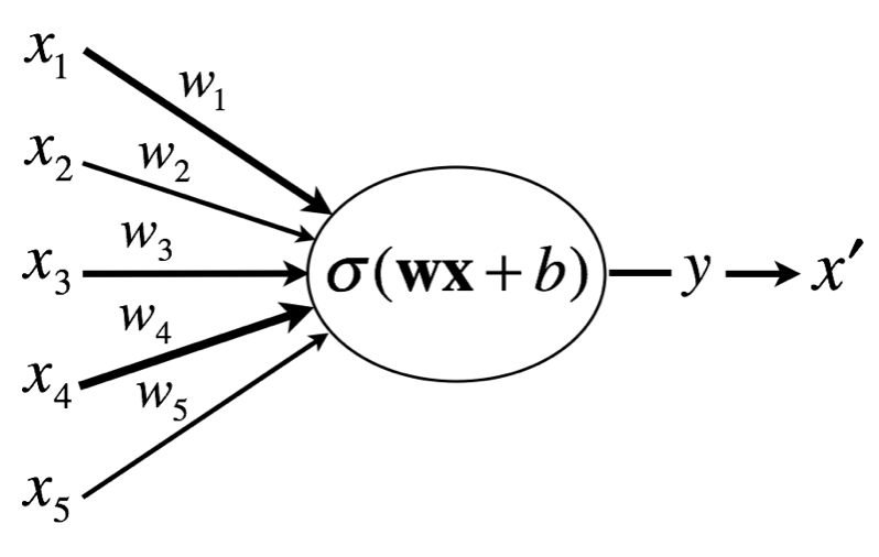
In neural network, an output of linear (fully connected) layer before being subjected to activation function is frequently said to be the logit, because the linear layer performs the logistic regression.
\[\text{logit}(\mathbf{x}) = \text{log}\frac{p(\mathbf{x})}{1-p(\mathbf{x})} := w_1x_1 + w_2x_2 + ... + w_nx_n + b = \mathbf{w}\mathbf{x}+b\]
Considering that the bias term (intercept) \(b=w_0\) is independent from data term \(x_i\), the bias term can be viewed as log prior odds and the weighted sum of \(x_i\), \(\mathbf{w}\mathbf{x}\), can be viewed as log likelihood ratio. Thus, if we think outputs (\(\mathbf{x}\)) of preceding nodes as feature values, neurons calculate logit (as a sum of log likelihood ratios, \(\Sigma\), and log prior odds, \(b\)) from them and returns posterior probability, which will be received as a feature value by the succeeding neuron.
\[\begin{equation} \begin{aligned} \Sigma &= \mathbf{w}\mathbf{x} \\ \psi &= \Sigma + b \\ y &= \sigma(\psi) \\ x^{'} &= y \end{aligned} \end{equation}\]