Probability and Random Variable
You may have heard of Schrödinger’s cat mentioned in a thought experiment in quantum physics. Briefly, according to the Copenhagen interpretation of quantum mechanics, the cat in a sealed box is simultaneously alive and dead until we open the box and observe the cat. The macrostate of cat (either alive or dead) is determined at the moment we observe the cat. Although not directly applicable, I think the indeterminacy of macrostate in quantum mechanics has some analogy to random variable in probability theory in that the value (\(x\)) of the random (\(X\)) is determined at the moment the random is observed and we say \(x\) is the realization of \(X\). Before we begin, let’s define some terms used in probability theory.
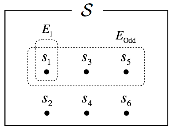
An experiment is the process by which an observation is made, and the experiment results in one or more outcomes, which are called events. If the experiment is die-tossing, event can be an observation of a 1 \((E_1)\) or an observation of odd number \((E_O)\). You may notice that \(E_O\) can be decomposed into an observation of 1 \((E_1)\), 3 \((E_3)\), or 5 \((E_5)\). The event that cannot be decomposed is called a simple event, and the event that can be decomposed into simple events is called a compound event. With the view of set theory, the simple event corresponds to one sample point \((s)\) in a sample space \((S)\), a set consisting of all possible sample points. \(S\) can contain a finite (or countably infinite) number of sample points or infinite number of sample points; the former is called discrete sample space and the latter is called continuous sample space. For a while, I will only use discrete sample space for simplicity. Thus, formally, an event in a discrete sample space is a collection of sample points, which is any subset of \(S\).
Probability
Now, let's think of probability. What is a probability? There are many different definitions of probability including philosophical definitions. Among them, I will use two definitions: frequentist's and Bayesian.
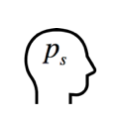
Suppose that there is a coin and you need to know the probability of observing head \((p_H)\) when you toss this coin one time. A conventional way to determine \(p_H\) is to toss the coin many times and use the frequency that heads are observed. If you calculate \(p_H\) using such approach, you are using the frequentist’s definition of probability. Let’s call \(p_s\) the point probability, that is the probability of sample point \(s\) (simple event). Then, the frequentist’s definition of is as follows:
\[p_s \triangleq \text{lim}_{N \rightarrow \infty} \frac{n_s}{N}\]
It is the relative proportion of times observing simple event \((n_s)\) in infinite number of trials \((N \rightarrow \infty)\). Thus, for frequentist's \(p_s\) to be valid (at least to be accurate to some degree), \(N\) should be very large. On the other hand, Bayesian definition of probability is just one’s belief on how likely an event occurs.
You may first think that Bayesian definition of probability is not scientific, since subjectivity cannot be introduced into the scientific inference. It is true that Bayesian probability is subjective, and because of such subjectivity Bayesian were scorned in the past. However, people disregarded an important point in Bayesian probability theory that probability (belief) updates when data (evidence) is encountered. I will further explain Bayesian updates latter. In the remaining part of this article, I will only use frequentist's definition of probability.
Now, let’s define a probability function \(P\). \(P\) takes an event (or events) as an input and returns the probability of the event(s). By using the definitions we have made so far, the probability of event(s) is as follows:
\[P(E) = \sum_{s \in E} p_s\]
Suppose that the experiment is tossing a coin three times (or tossing three coins). Then, the sample space of this experiment is as follows:
\[S = \{HHH, HHT, HTH, THH, TTH, THT, HTT, TTT \}\]
Assuming that the coin is perfectly balanced (i.e., \(p_H = p_T = \frac{1}{2}\)), each compound event is equally probable, that is
\[P_{HHH} = P_{HHT} = ... = P_{TTT} = \frac{1}{|S|} = \frac{1}{8}\]
As shown above, once the point probability is defined, calculation of the probability of event is just a matter of counting. For example, to calculate the probability of event \(A\) that we observe 2 heads in 3 coin-tosses, we only need to count the element in event \(A\).
\[A= \{HHT, HTH, THH\}\]
\[P(A) = p_{HHT} + p_{HTH} + p_{THH} = |A| \times \frac{1}{|S|} = 3 \times \frac{1}{8}\]
And there is a well-known counting method, called binomial coefficient, for the case when simple event is a binary outcome. The the number of ways of observing \(n_H\) heads in \(n\) coin-tosses (combinations) are calculated as follows.
\[\frac{n!}{n_H!(n-n_H)!} = \frac{(n_H+n_T)!}{(n_H)!(n_T)!}\]
Binomial coefficient actually calculates the number of ways of partitioning and is a special case of multinomial coefficient. By letting \(n = [n_1, n_2, ..., n_K]\), multinomial coefficient is defined as
\[M(\textbf{n}) = \frac{n!}{n_1!n_2!n_3!...n_K!} = \frac{(\sum_{k=1}^Kn_k)!}{n_1!n_2!n_3!...n_K!}\]
Random Variable
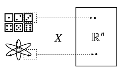
Now, consider event \(B\) = [1 head in 100 coin-tosses] or event \(C\) = [2 1s, 3 2s, 2 3s, 2 4s, 4 5s, 2 6s in 15 die-rolls]. Do we have to represent these events using sample points? Note that these events indicate the number of specific combinations of sample points. For example, if the number indicated by event is the number of heads in 3 coin-tosses, sample space \(S\) is reduced and mapped into other space \(\mathscr{X}\) (in this case subset of integers).
\[S = \{s_i\} = \{HH, HHT, HTH, THH, TTH, THT, HTT, TTT\}\]
\[\mathscr{X} = \{x_j\} = \{3,2,1,0\}\]
And we can think of a mapping function.
\[X: S \rightarrow \mathscr{X}\]
Thus, \(\mathscr{X}\) is the domain of the mapping function \(X\). For example, event \(A\) is mapped to integer 2.
\[X(A) = X(\{HHT, HTH, THH\}) = 2\in \mathscr{X}\]
We call the mapping function (usually denoted by upper case letter) random variable. As mentioned in the introduction, event can be viewed as an observed macrostate that is composed of microstate (sample points). And considering that the return value of random variable, \(x\), is a numerical representation of an event, the random variable is simultaneously in all possible macrostate (\(x \in \mathscr{X}\)) before the observation is made (\(X=x\)); \(x\) is also called realization of \(X\).
Random variables (hereafter, referred to as RV) are classified into two classes according to the properties of their domains: discrete RV and continuous RV. A RV \(X\) is said to be discrete if its domain is finite (e.g., \(\mathscr{X} = \{0,1,2\}\)) or countably infinite (e.g., \(\mathscr{X} = \mathbb{Z}^+\)), and a RV is said to continuous if its domain is uncountably infinite (e.g., \(\mathscr{X} = \mathbb{R}\)) (formally, continuous RV is defined as a RV with continuous cumulative distribution function). For example, the eye of a die is a discrete RV (\(\mathscr{X} = \{1,2,...,6\} \subset \mathbb{R}\)) and the position of an electron in 3D space is a continuous RV (\(\mathscr{X} = \mathbb{R}^3\)).
\(P\) returns the probability of an event. \(P\) can be used to get probability of the realization of discrete RV. In this case, the probability function is said to probability mass function (PMF).
\[p(x) = P(X =x)\]
Thus, the probability distribution for a discrete RV can be represented by a PMF for all \(x \in \mathscr{X}\) (or histogram). Using PMF, cumulative distribution function (CDF) is defined as follows:
\[F(x) = P(X \le x) = \sum_{t\le x}p(t)\]
For an RV that represents an eye of a balanced die, \(p(1) = P(X=1) = \frac{1}{6}\) and \(F(2) = P(X\le 2) = p(1) + p(2) = \frac{1}{3}\). Note that \(F(-\infty)=0\) and \(F(\infty)=1\).
What do you think of \(P(X=x)\) for continuous RVs? It may be counter-intuitive, but for continuous RVs, \(P(X=x)=0\) for all \(x \in \mathscr{X}\). You will see why this is true and why we use the term ’mass’ for discrete RVs. For continuous RVs, we first need to define probability density function (PDF). Suppose that there is a proper CDF for a continuous RV. Then PDF is defined as a derivative of CDF.
\[f(x) = F^{'}(x) = \frac{d F(x)}{d x}\]
Once PDF is defined, the probability (mass) for continuous RV is defined as an interval probability as follows:
\[P(a \le X \le) = \int_a^b f(x)dx\]
Thus, \(P(X=a) = P(a \le X \le a) = \int_a^a f(x) dx = 0\).
And since \(P(X=a)=0, P(a \le X \le b) = P(a < X \le b) = P(a < X < b)\). CDF can be obtained from PDF by integration.
\[F(x) = P(X\le x) = \int_{-\infty}^x f(t)dt\]
Expected Value of Random Variable
At this time, we need to define population and sample. The whole data that is the target of our interest is called the population and a subset selected from it is called sample. For example, if we want to make some inference on the hair length of Brown University students, whole set of hair length measurements is the population. It should be the best to make the inference using the whole data set (population), but a total inspection is costly and often impractical. An alternative way is that we collect the hair length measurements of a class of students and use this part (sample) of whole data set to make an inference on population.
The PMF and PDF are functions for describing population. If PMF or PDF of RV is available, it describes how the values of RV are distributed. And there are functions that summarize the distribution and tells us the shape of the distribution. The most frequently used values for describing the shape of the distribution is population mean and population variance. The former is frequently referred to as of RV and defined as follows:
\[E(X) = \left\{ \begin{array}{ll} \sum_x xp(x) \\ \int_x xf(x)dx \\ \end{array} \right.\]
Suppose that we are playing a coin-toss game (+1 point for head and 0 point for tail). After repeating the game 10 times, we collect a sample of 10 results. If the sample comprises seven +1s and three 0s, the mean score of the game will be calculated as follows
\[\bar{x} = \frac{1}{n}\sum_{i=1}^n x_i = \frac{1}{10}[(1 \times 7)+(0 \times 3)] = (1 \times \frac{7}{10}) + (0 \times \frac{3}{10}) = 0.7\]
Above is the way of calculating sample mean (with size \(n=10\)). Note that 7/10 and 3/10 are the relative proportions of heads and tails, respectively. What if the sample size is increased to \(n=\infty\)? Actually, the set of infinite number of measurements is the population. Also, the relative proportions of specific outcome in infinite number of trials is the probability. Thus, when calculating population mean (expected value), we use PMF. If \(p(1) = 0.65\) and \(p(0) = 0.35\), population mean is as follows:
\[E(X) = 1p(1) + 0p(1) = 1\times 0.65 + 0 \times 0.35 = 0.65\]
Population mean is denoted by \(\mu = E(X)\) (sample mean is the estimator of \(\mu\)). Why is the population mean called expected value? As mentioned earlier, the value of RV is determined at the moment of observation. But, with the expected value of RV (without observations), we can roughly imagine what the values of RV are. Suppose you are going out on a blind date. Before going out, you’ll probably have some expectation of the person coming. Assume for the sake of example that I’ve seen a lot of Brown University students whose hair length is 7 cm and I know in advance that the person whose coming to the blind date is from Brown University (meaning that you know the population mean is 7 cm). Then I will have some expectation that the person will have hair length of 7 cm.
There can be functions of RV, and the expected value of the function of RV is as follows:
\[E[g(X)] = \left\{ \begin{array}{ll} \sum_x g(x)p(x) \\ \int_x g(x)f(x)dx \\ \end{array} \right.\]
Variance of Random Variable
Continuing with the blind date example, although I expect that the person will have hair length of 7 cm, the person who comes may vary from my expectation and may have hair length of 4 cm! How can we express the possible variations from expectation (variation from expected value)? Let the function of RV as follows:
\[g(X) = [X-E(X)]^2 = (X-\mu)^2\]
Then the expected value of \(g(X)\) is the variance of RV \(X\).
\[V(X) = E[X-E(X)]^2 = E[(X-\mu)^2]\]
The expected value \(E(X)\) indicates the location of the population distribution and the variance \(V(X)\) indicates how much data points are dispersed from \(E(X)\). Thus, the lower the variance, the more you are confident that the person who will appear has hair length of 7 cm. The calculation of variance can be done more easily as follows:
\[\begin{equation} \begin{aligned} V(X) &= E[(X-\mu)^2]\\ &= E(X^2) - 2\mu E(X) + \mu^2 \\ &= E(X^2) - 2\mu^2 + \mu^2 \\ &= E(X^2) - \mu^2 \\ &= E(X^2) - [E(x)]^2 \\ \end{aligned} \end{equation}\]
Population variance is denoted by \(\sigma^2 = V(X)\). Sample variance is denoted by \(S^2\).
\[S^2 = \frac{1}{(n-1)}\sum_{i=1}^n (x_i - \bar{x})^2\]
The reason \((n-1)\) is used as a denominator instead of \(n\) as in the case of sample mean is to make \(S^2\) an unbiased estimate of \(\sigma^2\).